Download
1 / 29
290 likes | 338 Views
Discussing Bose-Einstein condensates (BEC) in random potentials, exploring interactions and coherence lengths. Examining Mott insulator, Bose glass, and Anderson localization phases, and quantum phase transitions in the presence of disorder.

E N D
LENS European Laboratory for Nonlinear Spectroscopy Università di Firenze J. E. Lye,, L. Fallani, M. Modugno, D. Wiersma, C. Fort, M. Inguscio Bose-Einstein condensates in random potentials Les Houches, February 2005
Outlook Why a random potential? How to produce a random potential First results from a BEC in a speckle potential Conclusions Chiara Fort Jessica Lye Leonardo Fallani Michele Modugno Massimo Inguscio Diederik Wiersma
Why random potentials? Examples of existing systems with random media Suppression of superfluidity of 4He in porous media with disorderAnderson Localisation of photons in strongly scattering semiconductor powders Disruption of electron transport due to defects in a solid – Anderson Localisation? Bose-Einstein condensates in random potentials … Long coherence length coupled with a controllable systemExploring the role of interactions without loss of coherence Control of dimensionalityEngineering new quantum phases (Bose glass) and Anderson localizationTransport/superfluid properties in the presence of disorder BEC in microtraps Fragmentation caused by imperfections of the microchipModification of superfluid properties?
Quantum phase transitions hopping energy interaction energy disorder D J U U J ei D At zero temperature, when quantum fluctuations become important, a BEC in an optical lattice in the tight-binding regime is well-described by the Bose-Hubbard model: Bose-Hubbard Hamiltonian
Superfluid/Mott insulator transition Quantum fluctuations can induce a phase transition from a superfluid phase to a Mott insulator phase. The transition is induced by a competition between two energy scales: hopping energy interaction energy < > J U U E • MOTT INSULATOR PHASE (U > J) • No phase coherence • Zero number fluctuations • Gap in the excitation spectrum • Vanishing superfluid fraction • SUPERFLUID PHASE ( J > U) • Long-range phase coherence • High number fluctuations • No gap in the excitation spectrum
Mott insulator / Bose Glass transition U E D With sufficient disorder, a quantum phase transition to the Bose Glass state occurs: disorder interaction energy hopping energy > > D U J • BOSE-GLASS PHASE (BG) • No phase coherence • Low number fluctuations • No gap in the excitation spectrum • Vanishing superfluid fraction • MOTT INSULATOR PHASE (MI) • No phase coherence • Zero number fluctuations • Gap in the excitation spectrum • Vanishing superfluid fraction
Anderson Localisation Scattering model Anderson Hopping model disorder hopping energy > D J D. Wiersma et al. Nature 390 671 (1997) • ANDERSON LOCALISATION • Long-range phase coherence • High number fluctuations • No gap in the excitation spectrum • Vanishing superfluid fraction • With sufficient scattering, the light waves can follow a random light path back to the source • The waves can propagate in two opposite directions along the looped path, each acquiring the same phase, and interfere constructively at the source, hence there is a higher probability of the wave returning to the source, and a lower probability of propagating away. * Phase coherence is maintained, but hopping is inhibited by lattice topology
Phase diagram • BOSE-GLASS PHASE (BG) • No phase coherence • Low number fluctuations • No gap in the excitation spectrum • Vanishing superfluid fraction • ANDERSON LOCALISATION • Long-range phase coherence • High number fluctuations • No gap in the excitation spectrum • Vanishing superfluid fraction (R. Roth and K. Burnett, PRA 68, 023604 (2003)) • MOTT INSULATOR PHASE (MI) • No phase coherence • Zero number fluctuations • Gap in the excitation spectrum • Vanishing superfluid fraction • SUPERFLUID PHASE • Long-range phase coherence • High number fluctuations • No gap in the excitation spectrum
A possible route to Bose-Glass… E First, to reach a Mott-Insulator phase with a regular lattice Second, to add disorder to the lattice B. Damski et al. PRL 91 080403 (2003) R. Roth and K. Burnett, PRA 68, 023604 (2003) The amount of disorder necessary to enter the Bose Glass phase is relatively small, being of the order of the interaction energy Or Anderson Localisation… Reduce interactions through expansion? in the random potential alone?
The random potential Two possible solutions to add disorder to the system: Speckle pattern Bichromatic lattice (pseudorandom)
Production of the random potential The random potential is produced by shining an off-resonant laser beam onto a diffusive plate and imaging the resulting speckle pattern on the BEC. speckle pattern BEC The BEC is illuminated by the speckle beam in the same direction as the imaging beam. With the same imaging setup we can detect both the BEC and the speckle pattern. 400 mm
What the random potential looks like FFT The speckle pattern is in good approximation a random “white” noise. However, due to the finite resolution of our system, the interspeckle distance starts from 10 mm. 9.6 mm 9.6 mm We define the average speckle height VSP as twice the standard deviation of the potential profile:
A comment • NOTE on length scales: • With a site separation of 10 mm, the tunnelling time in the tight binding limit is far greater than the time scale of the experiment, thus by simply increasing the height of the speckle potential alone we cannot reach the Bose Glass regime. • If the interactions are sufficiently low this could be a suitable length scale to see Anderson Localisation? • This length scale is comparable to that seen in microtrap experiments
Expansion from the speckle potential We adiabatically ramp the intensity of the speckle pattern on the trapped BEC, then we suddenly switch off both the magnetic trap and the speckle field and image the atomic cloud after expansion: VSP = 10 Hz VSP = 30 Hz speckle intensity VSP = 100 Hz Releasing the BEC from the weak speckle (VSP < m ~ 1kHz) potential we observe some irregular stripes in the expanded cloud. VSP = 200 Hz Releasing the BEC from the strong speckle (VSP > m) potential we observe the disappearance of the fringes and the appareance of a broader gaussian unstructured distribution. VSP = 2000 Hz
Expansion from the speckle potential In order to check if the observed density distribution was simply caused by heating, we have checked the adiabaticity of the procedure by applying a reverse ramp on the speckle intensity. A B C
Transport in the speckle potential Dipole mode Sudden displacement of the magnetic trap center along the x direction.
Interference from a finite number of point-like emitters Interference of an array of independent BECs Z. Hadzibabic et al., PRL 93 180403 (2004) • Detecting a Bose-Glass phase... • No interference fringes in a randomly spaced sample even without a phase transition Expansion of a coherent array of BECs P. Pedri et al., Phys. Rev. Lett. 87, 220401 (2001) Interference from randomly spaced BECs located at different sites high contrast regular spacing coherent sources lower contrast regular spacing incoherent sources no interference disorderd spacing coherent sources
Expansion from the speckle potential Observation of Phase Fluctuations in Elongated BECs S. Dettmer et al., Phys. Rev. Lett. 87, 160406 (2001) Dynamical instability of a BEC in a moving lattice L. Fallani et al., Phys. Rev. Lett. 93, 140406 (2004) No disorder VSP = 0 • Moderate disorder (VSP < m): • long wavelength modulations • breaking phase uniformity? • strong damping of the dipole mode speckle intensity VSP = 200 Hz • Strong disorder (VSP > m): • broad unstructured density profile because expansion from randomly spaced array • classically localized condensates in the speckles sites S VSP = 1700 Hz
Collective excitations in the random potential Quadrupole mode Resonant modulation of the radial trapping frequency (via the magnetic bias field) in the case of ordinary fluids: noninteracting gas Dipole mode Sudden displacement of the magnetic trap center along the x direction. strongly interacting gas peculiar of superfluid behavior After producing the BEC, we adiabatically load the BEC in the disordered potential Then we excite collective modes in the harmonic + random potential: ? ?
Collective excitations in the weak speckle potential We investigate the weak disorder regime, where the speckle field produces a weak perturbation of the harmonic trapping field and the system is not trapped in individual speckle wells. P = 5 mW VSP = 100 Hz m
Collective excitations in the weak speckle potential quadrupole (0 mW) quadrupole (2 mW) – VSP = 40 Hz dipole (0 mW) dipole (3 mW) – VSP = 60 Hz
Frequency shift in the quadrupole mode We see small frequency shifts to both the blue and the red, depending on the particular speckle realization, that becomes stronger increasing the speckle power.
Collective excitations in the weak speckle potential Using the sum-rules approach, and treating the speckle potential as a small perturbation : For a non-harmonic potential, shifts in the quadrupole frequency are not necessary correlated to shifts in the dipole frequency. This effect could mask any other possible changes in the excitation modes.
Summary How we produce a random potential Results from the BEC in a random potential Stripes in the density profile at moderate disorder, with strong damping of the dipole mode.Gaussian distribution at strong disorder, atoms classically localized in randomly spaced speckle wells.frequency shift of the quadrupole mode uncorrelated to a frequency shift in the dipole mode due to anharmonic speckle potential. Future projects Study of localization effects:Combining speckle potential with optical lattice standing wave: Mott-Insulator Bose GlassAnderson localization with speckle potential alone, reducing interactions through expansion
Observation of the Mott insulator phase (M. Greiner et al., Nature 415, 39 (2002)) The Mott insulator phase has been first obtained in a BEC trapped in a 3D optical lattice increasing the lattice height above a critical value Interference pattern of an interacting BEC released from a 3D optical lattice approaching the quantum transition: J decreases U increases Increasing the lattice height increases • Vanishing of 3D interference pattern loss of long range coherence, phase fluctuations • Applying a magnetic field gradient, the excitation spectrum was measured and the distinctive energy gap of the Mott-insulator was seen
Production of the random potential The random potential is produced by shining an off-resonant laser beam onto a diffusive plate and imaging the resulting speckle pattern on the BEC. stationary in time randomly varying in space Optical dipole potential