Chapter 14 Multiple Regression Analysis and Model Building

1. Business Statistics: A Decision-Making Approach 6th Edition Chapter 14Multiple Regression Analysis and Model Building

2. Chapter Goals After completing this chapter, you should be able to: • understand model building using multiple regression analysis • apply multiple regression analysis to business decision-making situations • analyze and interpret the computer output for a multiple regression model • test the significance of the independent variables in a multiple regression model

3. Chapter Goals (continued) After completing this chapter, you should be able to: • use variable transformations to model nonlinear relationships • recognize potential problems in multiple regression analysis and take the steps to correct the problems. • incorporate qualitative variables into the regression model by using dummy variables.

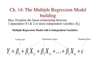
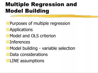
4. The Multiple Regression Model Idea: Examine the linear relationship between 1 dependent (y) & 2 or more independent variables (xi) Population model: Y-intercept Population slopes Random Error Estimated multiple regression model: Estimated (or predicted) value of y Estimated intercept Estimated slope coefficients

5. Multiple Regression Model Two variable model y Slope for variable x1 x2 Slope for variable x2 x1

6. Multiple Regression Model Two variable model y Sample observation yi < yi < e = (y – y) x2i x2 < x1i The best fit equation, y , is found by minimizing the sum of squared errors, e2 x1

7. Multiple Regression Assumptions • The errors are normally distributed • The mean of the errors is zero • Errors have a constant variance • The model errors are independent Errors (residuals) from the regression model: e = (y – y) <

8. Model Specification • Decide what you want to do and select the dependent variable • Determine the potential independent variables for your model • Gather sample data (observations) for all variables

9. The Correlation Matrix • Correlation between the dependent variable and selected independent variables can be found using Excel: • Tools / Data Analysis… / Correlation • Can check for statistical significance of correlation with a t test

10. Example • A distributor of frozen desert pies wants to evaluate factors thought to influence demand • Dependent variable: Pie sales (units per week) • Independent variables: Price (in $) Advertising ($100’s) • Data is collected for 15 weeks

11. Pie Sales Model Sales = b0 + b1 (Price) + b2 (Advertising) Multiple regression model: Correlation matrix:

12. Interpretation of Estimated Coefficients • Slope (bi) • Estimates that the average value of y changes by bi units for each 1 unit increase in Xi holding all other variables constant • Example: if b1 = -20, then sales (y) is expected to decrease by an estimated 20 pies per week for each $1 increase in selling price (x1), net of the effects of changes due to advertising (x2) • y-intercept (b0) • The estimated average value of y when all xi = 0 (assuming all xi = 0 is within the range of observed values)

13. Pie Sales Correlation Matrix • Price vs. Sales : r = -0.44327 • There is a negative association between price and sales • Advertising vs. Sales : r = 0.55632 • There is a positive association between advertising and sales

14. Scatter Diagrams Sales Sales Price Advertising

15. Estimating a Multiple Linear Regression Equation • Computer software is generally used to generate the coefficients and measures of goodness of fit for multiple regression • Excel: • Tools / Data Analysis... / Regression • PHStat: • PHStat / Regression / Multiple Regression…

16. Multiple Regression Output

17. The Multiple Regression Equation where Sales is in number of pies per week Price is in $ Advertising is in $100’s. b1 = -24.975: sales will decrease, on average, by 24.975 pies per week for each $1 increase in selling price, net of the effects of changes due to advertising b2 = 74.131: sales will increase, on average, by 74.131 pies per week for each $100 increase in advertising, net of the effects of changes due to price

18. Using The Model to Make Predictions Predict sales for a week in which the selling price is $5.50 and advertising is $350: Note that Advertising is in $100’s, so $350 means that x2 = 3.5 Predicted sales is 428.62 pies

19. Multiple Coefficient of Determination • Reports the proportion of total variation in y explained by all x variables taken together

20. Multiple Coefficient of Determination (continued) 52.1% of the variation in pie sales is explained by the variation in price and advertising

21. Adjusted R2 • R2 never decreases when a new x variable is added to the model • This can be a disadvantage when comparing models • What is the net effect of adding a new variable? • We lose a degree of freedom when a new x variable is added • Did the new x variable add enough explanatory power to offset the loss of one degree of freedom?

22. Adjusted R2 (continued) • Shows the proportion of variation in y explained by all x variables adjusted for the number of xvariables used (where n = sample size, k = number of independent variables) • Penalize excessive use of unimportant independent variables • Smaller than R2 • Useful in comparing among models

23. Multiple Coefficient of Determination (continued) 44.2% of the variation in pie sales is explained by the variation in price and advertising, taking into account the sample size and number of independent variables

24. Is the Model Significant? • F-Test for Overall Significance of the Model • Shows if there is a linear relationship between all of the x variables considered together and y • Use F test statistic • Hypotheses: • H0: β1 = β2 = … = βk = 0 (no linear relationship) • HA: at least one βi≠ 0 (at least one independent variable affects y)

25. F-Test for Overall Significance (continued) • Test statistic: where F has (numerator) D1 = k and (denominator) D2 = (n – k - 1) degrees of freedom

26. F-Test for Overall Significance (continued) With 2 and 12 degrees of freedom P-value for the F-Test

27. H0: β1 = β2 = 0 HA: β1 and β2 not both zero  = .05 df1= 2 df2 = 12 F-Test for Overall Significance (continued) Test Statistic: Decision: Conclusion: Critical Value: F = 3.885 Reject H0 at  = 0.05 The regression model does explain a significant portion of the variation in pie sales (There is evidence that at least one independent variable affects y)  = .05 0 F Do not reject H0 Reject H0 F.05 = 3.885

28. Are Individual Variables Significant? • Use t-tests of individual variable slopes • Shows if there is a linear relationship between the variable xi and y • Hypotheses: • H0: βi = 0 (no linear relationship) • HA: βi≠ 0 (linear relationship does exist between xi and y)

29. Are Individual Variables Significant? (continued) H0: βi = 0 (no linear relationship) HA: βi≠ 0 (linear relationship does exist between xi and y) Test Statistic: (df = n – k – 1)

30. Are Individual Variables Significant? (continued) t-value for Price is t = -2.306, with p-value .0398 t-value for Advertising is t = 2.855, with p-value .0145

31. H0: βi = 0 HA: βi 0 Inferences about the Slope: tTest Example From Excel output: • d.f. = 15-2-1 = 12 • = .05 t/2 = 2.1788 The test statistic for each variable falls in the rejection region (p-values < .05) Decision: Conclusion: a/2=.025 a/2=.025 Reject H0 for each variable There is evidence that both Price and Advertising affect pie sales at  = .05 Reject H0 Do not reject H0 Reject H0 -tα/2 tα/2 0 -2.1788 2.1788

32. Confidence Interval Estimate for the Slope Confidence interval for the population slope β1 (the effect of changes in price on pie sales): where t has (n – k – 1) d.f. Example: Weekly sales are estimated to be reduced by between 1.37 to 48.58 pies for each increase of $1 in the selling price

33. Standard Deviation of the Regression Model • The estimate of the standard deviation of the regression model is: • Is this value large or small? Must compare to the mean size of y for comparison

34. Standard Deviation of the Regression Model (continued) The standard deviation of the regression model is 47.46

35. Standard Deviation of the Regression Model (continued) • The standard deviation of the regression model is 47.46 • A rough prediction range for pie sales in a given week is • Pie sales in the sample were in the 300 to 500 per week range, so this range is probably too large to be acceptable. The analyst may want to look for additional variables that can explain more of the variation in weekly sales

36. R commands • paste("Today is", date()) • y=c(350, 460, 350, 430, 350, 380, 430, 470, 450, 490, 340, 300, 440, 450, 300) • #y is apple pie sales • x=c(5.5, 7.5, 8.0, 8.0, 6.8, 7.5, 4.5, 6.4, 7.0, 5.0, 7.2, 7.9, 5.9, 5.0, 7.0) • #price charged • z=c(3.3, 3.3, 3.0, 4.5, 3.0, 4.0, 3.0, 3.7, 3.5, 4.0, 3.5, 3.2, 4.0, 3.5, 2.7) • #advertising expenses • t.test(x); sort(x); t.test(y); sort(y) • t.test(z); sort(z) • library(fBasics)

37. R commands set 2 • cs=colStats(cbind(y,x,z), FUN=basicStats); cs • #following function automatically computes outliers • get.outliers = function(x) { • #function to compute the number of outliers automatically • #author H. D. Vinod, Fordham university, New York, 24 March, 2006 • su=summary(x) • if (ncol(as.matrix(x))>1) {print("Error: input to get.outliers function has 2 or more columns") • return(0)} • iqr=su[5]-su[2] • dn=su[2]-1.5*iqr • up=su[5]+1.5*iqr • LO=x[x<dn]#vector of values below the lower limit • nLO=length(LO) • UP=x[x>up] • nUP=length(UP) • print(c(" Q1-1.5*(inter quartile range)=", • as.vector(dn),"number of outliers below it are=",as.vector(nLO)),quote=F) • if (nLO>0){ • print(c("Actual values below the lower limit are:", LO),quote=F)} • print(c(" Q3+1.5*(inter quartile range)=", • as.vector(up)," number of outliers above it are=",as.vector(nUP)),quote=F) • if (nUP>0){ • print(c("Actual values above the upper limit are:", UP),quote=F)} • list(below=LO,nLO=nLO,above=UP,nUP=nUP,low.lim=dn,up.lim=up)} • #xx=get.outliers(x) • # function ends here = = = = = =

38. R commands set 3 • xx=get.outliers(x) • xx=get.outliers(y) • xx=get.outliers(z) • #Tests for Correlation Coefficients • cor.test(x,y) • #capture.output(cor.test(x,y), file="c:/stat2/PieSaleOutput.txt", append=T) • cor.test(z,y) • #capture.output(cor.test(z,y), file="c:/stat2/PieSaleOutput.txt", append=T) • cor.test(x,z) • #capture.output(cor.test(x,z), file="c:/stat2/PieSaleOutput.txt", append=T) • #Now regression analysis • reg1=lm(y~x+z) • summary(reg1) #plot(reg1) • library(car); confint(reg1) #prints confidence intervals

39. Multicollinearity • Multicollinearity: High correlation exists between two independent variables • This means the two variables contribute redundant information to the multiple regression model

40. Multicollinearity (continued) • Including two highly correlated independent variables can adversely affect the regression results • No new information provided • Can lead to unstable coefficients (large standard error and low t-values) • Coefficient signs may not match prior expectations

41. Some Indications of Severe Multicollinearity • Incorrect signs on the coefficients • Large change in the value of a previous coefficient when a new variable is added to the model • A previously significant variable becomes insignificant when a new independent variable is added • The estimate of the standard deviation of the model increases when a variable is added to the model

42. Detect Collinearity (Variance Inflationary Factor) VIFj is used to measure collinearity: R2j is the coefficient of determination when the jth independent variable is regressed against the remaining k – 1 independent variables If VIFj > 5, xj is highly correlated with the other explanatory variables

43. Detect Collinearity in PHStat Output for the pie sales example: • Since there are only two explanatory variables, only one VIF is reported • VIF is < 5 • There is no evidence of collinearity between Price and Advertising • PHStat / regression / multiple regression … • Check the “variance inflationary factor (VIF)” box

44. Qualitative (Dummy) Variables • Categorical explanatory variable (dummy variable) with two or more levels: • yes or no, on or off, male or female • coded as 0 or 1 • Regression intercepts are different if the variable is significant • Assumes equal slopes for other variables • The number of dummy variables needed is (number of levels - 1)

45. Dummy-Variable Model Example (with 2 Levels) Let: y = pie sales x1 = price x2 = holiday (X2 = 1 if a holiday occurred during the week) (X2 = 0 if there was no holiday that week)

46. Dummy-Variable Model Example (with 2 Levels) (continued) Holiday No Holiday Different intercept Same slope y (sales) If H0: β2 = 0 is rejected, then “Holiday” has a significant effect on pie sales b0 + b2 Holiday b0 No Holiday x1 (Price)

47. Interpretation of the Dummy Variable Coefficient (with 2 Levels) Example: Sales: number of pies sold per week Price: pie price in $ Holiday: 1 If a holiday occurred during the week 0 If no holiday occurred b2 = 15: on average, sales were 15 pies greater in weeks with a holiday than in weeks without a holiday, given the same price

48. Dummy-Variable Models (more than 2 Levels) • The number of dummy variables is one less than the number of levels • Example: y = house price ; x1 = square feet • The style of the house is also thought to matter: Style = ranch, split level, condo Three levels, so two dummy variables are needed

49. Dummy-Variable Models (more than 2 Levels) (continued) Let the default category be “condo” b2 shows the impact on price if the house is a ranch style, compared to a condo b3 shows the impact on price if the house is a split level style, compared to a condo

50. Interpreting the Dummy Variable Coefficients (with 3 Levels) Suppose the estimated equation is For a condo: x2 = x3 = 0 With the same square feet, a split-level will have an estimated average price of 18.84 thousand dollars more than a condo For a ranch: x3 = 0 With the same square feet, a ranch will have an estimated average price of 23.53 thousand dollars more than a condo. For a split level: x2 = 0