Download
1 / 21
230 likes | 442 Views
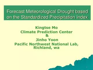
Forecast Meteorological Drought based on the Standardized Precipitation Index. Kingtse Mo Climate Prediction Center & Jinho Yoon Pacific Northwest National Lab, Richland, wa. Objectives. Develop objective drought Prediction based on drought indices

E N D
Forecast Meteorological Drought based on the Standardized Precipitation Index Kingtse Mo Climate Prediction Center & Jinho Yoon Pacific Northwest National Lab, Richland, wa
Objectives • Develop objective drought Prediction based on drought indices • Meteorological drought: based on the Precipitation deficit. Index: Standardized Precipitation Index (SPI)
SPI SPI3-SPi12: For drought monitoring: SPIs are updated daily using the CPC unified Precip analysis Advantages: Only need precipitation Can be applied to station data SPI3: shorter range P conditions SPI6 comparable time scales with soil moisture SPi12-24: long term drought D3 D2 D1
Predicting SPI from CFS over the United States Downscaling from the CFS forecasts (T62) to 50 KM. Four different downscaling methods are tested Append the corrected P forecasts to the observed P data set Compute SPI from 3 months to 12 months Evaluate the forecasts
Bilinear interpolation Correct the model climatology and bilinear interpolation to a high resolution grid Example: 1988 Nov Ensemble CFS T62 fcsts • Too smooth over the mountain region, • amplitudes are too low because of ensemble mean , low resolution,and BI
Bias correction & Downscaling (BCSD) Probability mapping based on distributions • Get probability distribution PDFs for A (coarse T62 fcsts ) and A(fine, obs) • From A (coarse) get percentile based on PDF (coarse) • => assume the same percentile for the fine grid and work backward based on the PDF fine get A fine (anomaly) • If normally distributed , time ratio of std Ref Wood et al (U. Washington 2002,2006)
1988 Nov Improvements over mountain regions stronger amplitudes
Schaake’s linear regression • Schaake’s linear regression – calibrate P ensemble forecasts based on the historical performance • For P, transfer to normal space first r Can be negative=>make fcsts worse Ref: Wood and Schaake (2008) Schaake et al. (2007)
Bayesian merging & bias correction • Bayesian correction – calibrate Probability distribution based on forecast information • Calibration based on the linear regression fcst=a*obs+b and spread Ref: Luo et al. (2007); Luo and Wood (2008)
Bayesian method For T62 CFS forecasts, the spread is large because of low skill and ICs cover large interval (about 25 days apart) Amplitudes of forecasts after Bayesian downscaling are too weak. Here, we use no spread (Coelho et al. 2004), but screen to select only fcsts close to the ensemble mean
1988 Nov A good fcst Spread is too large, so it dumps fcst. Magnitudes are too weak Screen fcsts No spread
Nov May P Correlationfor lead=1 BCSD Schaake Bayesian Ensemble
Standardized Precipitation Index Forecasts • Append the bias corrected and downscaled P to the observed P time series • Calculate SPI from extended time series • The advantages are (1) no need of hydrologic model and (2) can use any base period. • An example: Fcst Nov 1981 SPIs P : observed : Jan1950-oct1981 append fcsts with ICs in Oct-Nov lead 1 f1 lead 2 f2 to f9 etc P time series: Jan1950-oct 1981 (obs) Nov 1981 (fcst) For SPI6 lead 1, there are 5 months of observed P
NOV 1.For the first 3 months, AC>0.6 and RMS < 0.8 2. From lead 1 to 4 mo, the fcsts are skillful and differences between downscaling methods are small. 3. Large differences occur after lag 4 when skill is low Seasonal dependence of skill FEB MAY BCSD Schaake Bayesian Ensemble mean Aug
rmes skill for different methods (may fcsts spi6) BCSD Schaake Bayesian lead1 Lead 2 Lead 3
RMSE Lead 1 Lead 2 SPI6-Bayesian Nov Feb May Aug
Dynamic downscaling based on the 50-km RSM • RSM (regional spectral model) nested in the CFS forecasts to downscale(April 28-May 3) ICs (50 km resolution) (Thanks, Henry Juang) • How does this compare with the statistical BCSD downscaling method
Correlation P SPI6 RSM-50km T62 BCSD 15mem RSM better than 5 mem, but worse than 15mem T62 T26 BCSD 5mem
Conclusions • Attempt has been made to predict the meteorological drought based on SPI from downscaled P from T62 CFS seasonal forecasts • 2. For SPI3, the ACC is above 0.5 for 2 months and for SPI6, the ACC is above 0.5 for 4 months. • For SPI prediction, the skill is not sensitive to the downscaling methods. • Dynamic downscaling based on the 50-RSM does not have advantage in comparison with the simple BCSD downscaling.