Download
1 / 27
280 likes | 405 Views
This presentation explores key advancements in neural network models beyond the simplistic perceptron activation function. We address common limitations such as the need for more input connections and the overly simplistic outputs produced by traditional perceptrons. The use of more complex activation functions, including sigmoid and logistic functions, are introduced to create more realistic neuronal behavior. We also delve into automatic training methods, particularly Rosenblatt’s training algorithm, providing a clear overview of adjustments made based on feedback to improve output accuracy.

E N D
Introduction to Training and Learning in Neural Networks • CS/PY 399 Lab Presentation # 4 • February 1, 2001 • Mount Union College
More Realistic Models • So far, our perceptron activation function is quite simplistic • f (x1 , x2 ) = 1, if xk·wk> , or • = 0, if xk·wk < • To more closely mimic actual neuronal function, our model needs to become more complex
Problem # 1: Need more than 2 input connections • addressed last time: activation function becomes f (x1 , x2 , x3 , ..., xn ) • vector and summation notation help with writing and describing the calculation being performed
Problem # 2: Output too Simplistic • Perceptron output only changes when an input, weight or theta changes • Neurons don’t send a steady signal (a 1 output) until input stimulus changes, and keep the signal flowing constantly • Action potential is generated quickly when threshold is reached, and then charge dissipates rapidly
Problem # 2: Output too Simplistic • when a stimulus is present for a long time, the neuron fires again and again at a rapid rate • when little or no stimulus is present, few if any signals are sent • over a fixed amount of time, neuronal activity is more of a firing frequency than a 1 or 0 value (a lot of firing or a little)
Problem # 2: Output too Simplistic • to model this, we allow our artificial neurons to produce a graded activity level as output (some real number) • doesn’t affect the validity of the model (we could construct an equivalent network of 0/1 perceptrons) • advantage of this approach: same results with smaller network
Output Graph for 0/1 Perceptron 1 output 0 θ Σ xk · wk
LIMIT function: More Realism • Define a function with absolute minimum and maximum output values (say 0 and 1) • Establish two thresholds: lower and upper • f (x1 , x2 , ..., xn ) = 1, if xk·wk>upper, • = 0, if xk·wk<lower, or • some linear function between 0 and 1, otherwise
Output Graph for LIMIT function 1 output 0 θlower θupper Σ xk · wk
Sigmoid Ftns: Most Realistic • Actual neuronal activity patterns (observed by experiment) give rise to non-linear behavior between max & min • example: logistic function • f (x1 , x2 , ..., xn ) = 1 / (1 + e- xk·wk), where e 2.71828... • example: arctangent function • f (x1 , x2 , ..., xn ) = arctan( xk·wk) / ( / 2)
Output Graph for Sigmoid ftn 1 output 0 0 Σ xk · wk
TLearn Activation Function • The software simulator we will use in this course is called TLearn • Each artificial neuron (node) in our networks will use the logistic function as its activation function • gives realistic network performance over a wide range of possible inputs
TLearn Activation Function • Table, p. 9 (Plunkett & Elman) InputActivationInputActivation -2.00 0.119 0.50 0.622 -1.50 0.182 1.00 0.731 -1.00 0.269 1.50 0.818 -0.50 0.378 2.00 0.881 0.00 0.500
TLearn Activation Function • output will almost never be exactly 0 or exactly 1 • reason: logistic function approaches, but never quite reaches these maximum and minimum values, for any input from - to • limited precision of computer memory will enable us to reach 0 and 1 sometimes
Automatic Training in Networks • We’ve seen: manually adjusting weights to obtain desired outputs is difficult • What do biological systems do? • if output is unacceptable (wrong), some adjustment is made in the system • how do we know it is wrong? Feedback • pain, bad taste, discordant sound, observing that desired results were not obtained, etc.
Learning via Feedback • Weights (connection strengths) are modified so that next time the same input is encountered, better results may be obtained • How much adjustment should be made? • different approaches yield various results • goal: automatic (simple) rule that is applied during weight adjustment phase
Rosenblatt’s Training Algorithm • Developed for Perceptrons (1958) • illustrative of other training rules; simple • Consider a single perceptron, with 0/1 output • We will work with a training set • a set of inputs for which we know the correct output • weights will be adjusted based on correctness of obtained output
Rosenblatt’s Training Algorithm • for each input pattern in the training set, do the following: • obtain output from perceptron • if output is correct: (strengthen) • if output is 1, set w = w + x • if output is 0, set w = w - x • but if output is incorrect: (weaken) • if output is 1, set w = w - x • if output is 0, set w = w + x
Example of Rosenblatt’s Training Algorithm • Training data: x1x2out 0 1 1 1 1 1 1 0 0 • Pick random values as starting weights and θ: w1 = 0.5, w2 = -0.4, θ = 0.0
Example of Rosenblatt’s Training Algorithm • Step 1: run first training case through a perceptron x1x2out 0 1 1 • (0, 1) should give answer 1 (from table), but perceptron produces 0 • do we strengthen or weaken? • do we add or subtract? • based on answer produced by perceptron!
Example of Rosenblatt’s Training Algorithm • obtained answer is wrong, and is 0: we must ADD input vector to weight vector • new weight vector: (0.5, 0.6) • w1 = 0.5 + 0 = 0.5 • w2 = -0.4 + 1 = 0.6 • Adjust weights in perceptron now, and try next entry in training data set
Example of Rosenblatt’s Training Algorithm • Step 2: run second training case through a perceptron x1x2out 1 1 1 • (1, 1) should give answer 1 (from table), and it does! • do we strengthen or weaken? • do we + or -?
Example of Rosenblatt’s Training Algorithm • obtained answer is correct, and is 1: we must ADD input vector to weight vector • new weight vector: (1.5, 1.6) • w1 = 0.5 + 1 = 1.5 • w2 = 0.6 + 1 = 1.6 • Adjust weights, then on to training case # 3
Example of Rosenblatt’s Training Algorithm • Step 3: run last training case through the perceptron x1x2out 1 0 0 • (1, 0) should give answer 0 (from table); does it? • do we strengthen or weaken? • do we + or -?
Example of Rosenblatt’s Training Algorithm • determine what to do, and calculate a new weight vector • should have SUBTRACTED • new weight vector: (0.5, 1.6) • w1 = 1.5 - 1 = 0.5 • w2 = 1.6 - 0 = 1.6 • Adjust weights, then try all three training cases again
Ending Training • This training process continues until: • perceptron gives correct answers for all training cases, or • a maximum number of training passes has been carried out • some training sets may be impossible for a perceptron to calculate (e.g., XOR ftn.) • In actual practice, we train until the error is less than an acceptable level
Introduction to Training and Learning in Neural Networks • CS/PY 399 Lab Presentation # 4 • February 1, 2001 • Mount Union College