Download
1 / 27
270 likes | 475 Views
Estimating CAPM Inputs. Where do r f , Beta, and T C Come From?. Estimating Betas. Comparable firm or industry method Regress rates of return on common stock against the rates of return on a “market” index. Normally we try to reduce the noise in betas by calculating industry betas.

E N D
Estimating CAPM Inputs Where do rf, Beta, and TC Come From?
Estimating Betas • Comparable firm or industry method • Regress rates of return on common stock against the rates of return on a “market” index. • Normally we try to reduce the noise in betas by calculating industry betas. • This is simply the average of all of the equity betas for firms within the industry.
Estimation Details • Daily, weekly, monthly or annual returns? • In the ideal world of the CAPM, without transactions costs, it does not matter. • In the real world with bid-ask spreads it does. • Investors buy stocks at the ask and sell them at the bid. The difference is the bid-ask spread and allows the market maker to earn a living. • Even absent any movement in a stock’s value, its price may change from day to day as the reported closing transaction bounces from the bid to the ask. • Bid-ask bounce makes it appear that movements in a stock are unrelated to the market. • Monthly returns minimize the impact of bid-ask bounce. • If your data set is to short to use monthly returns go to weekly. If it is too short for that . . . Best of luck.
More Estimation Details • What time period? • Try to use 60 periods of data. Yes, that would be five years of monthly data. • Are dividends and rights included in rates of return? • The holding period return should include ALL cash flows. If you can spend it, you should include it. • The initial cash outflow is the purchase price. • The final cash inflow is the sales price.
The Final Estimation Details • Which is the correct market index? • The CAPM market index includes all risky assets. • In theory this means you want the index of everything. • In practice this index does not exist. Even if it did you cannot own it as it includes items like real estate (your house), and human capital (you). • Wilshire 5000 comes close (^DWC). • CRSP index is similar (posted on the class web page) and includes all stocks on the NASDAQ, AMEX, and NYSE.
One Final Beta Estimator • Old joke: All betas equal one plus or minus estimation error. • There is a lot of truth to this crack. • Out of sample firms with low beta estimates tend to have unexpectedly high return correlations with the market. The reverse is true too. • On average betas have to equal one. Why not use this value absent convincing evidence to the contrary?
The Risk Free RateNo Easy Answers • Technical answer. • The mathematical models used to generate the intertemporal CAPM includes a risk free asset that pays an instantaneous interest rate rf. • Based on this you want the interest rate on a short dated treasury instrument. • But, these are stationary models. Things like inflation are not expected to change over time. • Still there is evidence that this is your best estimate of the long run risk free rate. • Out of sample economic models do a very poor job of predicting interest rates. Best model is typically that next year’s rate will equal this year’s rate.
Risk Free Rate Continued • Intuitive Answer • Use a ten year treasury rate. • Allows for changing returns over time. • Problems • Return from holding short dated government bonds over ten years. Think of buying one year bonds every year for ten years. • Return from holding a single ten year bond. • Single ten year bond has on average a higher return. This means the long dated bond returns include a risk premium. We want the risk free rate. • Partial solution: subtract out the historical risk premium of about 1%.
Risk Free Rate Continued • Not intuitive and not easy answer. • Calculate the forward rates from government bonds. Use these forward rates as your risk free rate. • Good • Allows for time variation in interest rates. • Bad • Forward rates more than a year out are likely to include a risk premium. • Pain in the neck to do this, often with only a minor impact to the final calculated value. • One of Many Possible Compromises • Use the five year bond’s return for your projected cash flows. • Use the ten year bond’s return for your terminal value’s cash flows.
Market Risk Premium • Another difficult and controversial topic. • The argument for 4%. • Given today’s market, and the historical growth in GDP it is hard to imagine a world in which stocks return more than 4% forever. • The argument for 7%. • This is the historical value. • The 4% argument could have been made many times in the past. It has yet to describe the market. • The argument for values in between. • I hate fighting, how about we all compromise on . . .
Estimating rD and βD • Just how accurate a number do you need? • Not very? Use either: • Last year’s interest payments divided by the outstanding debt. • The current yield to maturity its debt. • Set βD to zero. • What can go wrong? • How risky is the debt? • Not very? Then not much. Use one of the above estimates.
Estimating rD • No public debt? Call the bank! • Alternatively, go to their financial statements and use the interest paid divided by the outstanding debt. • With public debt. • Start with the yield to maturity of the bonds. • Adjust this for the chance the company will default on the bonds. • Use historical estimates to do the adjustment.
Risky Debt • The firm’s debt is very risky? • If there is a reasonable chance the firm will default then the interest rate on the firm’s debt will overestimate rD. • Investors will demand a higher promised yield to compensate them for those times when the firm fails to pay in full. • βD will have the same sign as βA.
How Risky is Risky?Bond Ratings • Major rating agencies: • Moody’s • S&P • Fitch • General categories • Investment grade (a.k.a. high grade) • BBB rating and higher. • High yield (a.k.a. junk) • Not investment grade, and not in default. • Distressed • In default
Historical Bond Returns and YieldsAverages for 1989-2003 Key: ML = Merrill Lynch, LB = Lehman Brothers, Yld = Yield to Maturity, TR = Total Return
Items to Note • Yield and total return are not the same thing! • Question: Why is the total return on treasuries higher than the yield? • Question: Why is this relationship reversed for CCC bonds? • The lower the corporate bond class rating the higher the yield. • The lower the corporate bond class rating the sometimes higher, sometimes lower the total return. • A table with the year by year data is on the class web page.
Adjusting rD for Default Risk • The return on the firm’s debt is equivalent the total return in the table. • Problem: You have yield to maturity data not expected return data. • One possible solution: Adjust the YTM using the historical relationship between YTM and rD based on the firm’s debt’s rating class.
A Warning • The data on the web page is from 1989-2003, which includes a very long economic boom. • During booms high yield debt should produce a return higher than investors expected. • During busts the opposite is true. • Are the 1989-2003 averages reflective of what investors expected?
Long Run Bond ReturnsDecember 1926 – December 1989 Key: Yld = Yield to Maturity, TR = Total Return
Long Run Results • Contrasts with data from 1989-2003 • For the long run data the AA and BAA bonds have higher YTM’s than TR’s. As expected. • For the 1989-2003 data the AA and BAA bonds have lower YTM’s than TR’s. Probably due to the long economic boom. • Lower credit quality bonds have higher total returns. • Another item to note: AA TR’s have been lower than government TR’s! Very odd. • The underlying data for the long run table is on the class web page.
Estimating TC • Use the average U.S. combined federal and state rate of 40%. • Use the value management provides. • Matt’s never before seen method!
Average U.S. Combined Rate • The average combined federal and state tax rate is 40%. • Good for primarily domestic firms that have been profitable. • Good long run value for firms you believe will become profitable. • Bad for firms with current or recent losses that may have tax loss carry forwards. • Potentially bad for firms with large foreign operations or overseas “headquarters.”
Management’s Reported Value • In the firm’s financial reports management will often provide their firm’s tax rate for the previous period. • This is often calculated as: 1- Net Income After Taxes/Net Income Before Taxes.
Management Reports: Good and Bad • Often accurate since management has access to the proprietary information provided to the IRS for calculating their taxes. • Good: Net Income numbers may provide an accurate picture of the marginal tax rate. • Bad: Net Income numbers are not cash flows and may not reflect the firm’s marginal or even average tax rate. • May not reflect future tax rates for firm’s that have been unprofitable but are now becoming profitable.
Matt’s Never Seen Before Method • Calculate the annual tax rate as the Cash Taxes Paid/FCF Before Taxes. • Use the average of the above from at least five years of data.
Matt’s Method: Good and Bad • Good: Uses only cash flow numbers. • Good: Over the “long run” this is the fraction of the firm’s free cash flow the government keeps. • Theoretically the number you want if this is the expected marginal tax rate going forward. • Bad: Very volatile. Tax rates will appear to jump dramatically from year to year. • Averaging helps quite a bit but with only five to ten data points perhaps not enough. • Bad: May not reflect future tax rates for firm’s that have been unprofitable but are now becoming profitable.
Combining the Best of All Methods • Goal: Obtain the firm’s tax rate in the years ahead. • Problem: Must use past data. • Solution: Project based on trends. • Recently unprofitable firms will have relatively low tax rates for at least the next few years as they use up their tax loss carry forwards. • Once a firm uses up its tax loss carry forwards expect its tax rate to approach 40% or its industry average. • Recently profitable firms will likely have the same tax rate going forward.