Download
1 / 34
340 likes | 393 Views
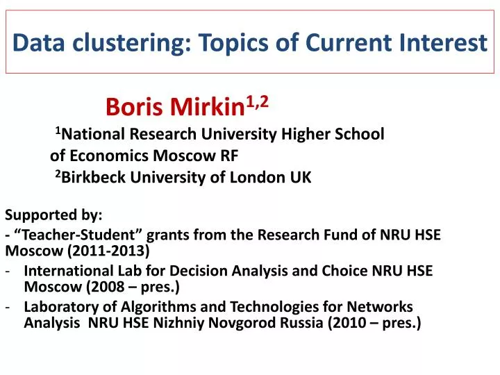
Data clustering: Topics of Current Interest. Boris Mirkin 1,2 1 National Research University Higher School of Economics Moscow RF 2 Birkbeck University of London UK Supported by: - “Teacher-Student” grants from the Research Fund of NRU HSE Moscow (2011-2013)

E N D
Data clustering: Topics of Current Interest Boris Mirkin1,2 1National Research University Higher School of Economics Moscow RF 2Birkbeck University of London UK Supported by: - “Teacher-Student” grants from the Research Fund of NRU HSE Moscow (2011-2013) International Lab for Decision Analysis and Choice NRU HSE Moscow (2008 – pres.) Laboratory of Algorithms and Technologies for Networks Analysis NRU HSE Nizhniy Novgorod Russia (2010 – pres.)
Data clustering: Topics of Current Interest K-Means clustering and two issues Finding right number of clusters Before clustering (anomalous) While clustering (divisive no minima of density function) Weighting features (3-step iterations) K-Means at similarity clustering (kernel k-means) Semi-average similarity clustering Consensus clustering Spectral clustering, Threshold clustering and Modularity clustering Laplacian pseudo-inverse transformation Conclusion
Batch K-Means: a generic clustering method Entities are presented as multidimensional points (*) 0. Put K hypothetical centroids (seeds) 1. Assign points to the centroids according to minimum distance rule 2. Put centroids in gravity centres of thus obtained clusters 3. Iterate 1. and 2. until convergence K= 3 hypothetical centroids (@) • * * • * * * * * • * * * • @ @ • @ • ** • * * *
K-Means: a generic clustering method Entities are presented as multidimensional points (*) 0. Put K hypothetical centroids (seeds) 1. Assign points to the centroids according to Minimum distance rule 2. Put centroids in gravity centres of thus obtained clusters 3. Iterate 1. and 2. until convergence • * * • * * * * * • * * * • @ @ • @ • ** • * * *
K-Means: a generic clustering method Entities are presented as multidimensional points (*) 0. Put K hypothetical centroids (seeds) 1. Assign points to the centroids according to Minimum distance rule 2. Put centroids in gravity centres of thus obtained clusters 3. Iterate 1. and 2. until convergence • * * • * * * * * • * * * • @ @ • @ • ** • * * *
K-Means: a generic clustering method Entities are presented as multidimensional points (*) 0. Put K hypothetical centroids (seeds) 1. Assign points to the centroids according to Minimum distance rule 2. Put centroids in gravity centres of thus obtained clusters 3. Iterate 1. and 2. until convergence 4. Output final centroids and clusters * * @ * * * @ * * * * ** * * * @
K-Means criterion: Summary distance to cluster centroids Minimize * * @ * * * @ * * * * ** * * * @
Advantages of K-Means - Models typology building - Simple “data recovery” criterion - Computationally effective - Can be utilised incrementally, `on-line’ Shortcomings of K-Means - Initialisation: no advice on K or initial centroids - No deep minima - No defence of irrelevant features
Issue: How the number and location of initial centers should be chosen? (Mirkin 1998, Chiang and Mirkin 2010) Equivalent criterion: Maximize where Nk is the number of entities in Sk <ck, ck> - Euclidean squared distance between 0 and ck Minimize • over S and c. • Data scatter (the sum • of squared data entries)= • = W(S,c)+D(S,c) • Data scatter is constant while partitioning CODA Week 8 by Boris Mirkin
Issue: How the number and location of initial centers should be chosen? 2 Maximize where Nk=|Sk| Preprocess data by centering: 0 is grand mean <ck, ck> - Euclidean squared distance between 0 and ckLook for anomalous & populated clusters!!! Further away from the origin. CODA Week 8 by Boris Mirkin
Issue: How the number and location of initial centers should be chosen? 3 Preprocess data by centering to Reference point, typically grand mean. 0 is grand mean since that. Build just one Anomalous cluster. CODA Week 8 by Boris Mirkin
Issue: How the number and location of initial centers should be chosen? 4 Preprocess data by centering to Reference point, typically grand mean. 0 is grand mean since that. Build Anomalous cluster: 1. Initial center c is entity farthest away from 0. 2. Cluster update.if d(yi,c) < d(yi,0), assignyi to S. 3. Centroid update: Within-Smean c'if c' c. Go to 2 with cc'. Otherwise, halt. CODA Week 8 by Boris Mirkin
Issue: How the number and location of initial centers should be chosen? 5 Anomalous Cluster is (almost) K-Means up to: (i) the number of clusters K=2: the “anomalous” one and the “main body” of entities around 0; (ii) center of the “main body” cluster is forcibly always at 0; (iii) a farthest away from 0 entity initializes the anomalous cluster. CODA Week 8 by Boris Mirkin
Issue: How the number and location of initial centers should be chosen? 6 Anomalous Cluster iK-Means is superior of: (Chiang, Mirkin, 2010) CODA Week 8 by Boris Mirkin
Issue: Weighting features according to relevance and Minkowski -distance (Amorim, Mirkin, 2012) • w: feature weights=scale factors • 3-step K-Means: • Given s, c, find w (weights) • Given w, c, find s (clusters) • Given s,w, find c (centroids) • till convergence
Issue: Weighting features according to relevance and Minkowski -distance 2Minkowski’s centers • Minimize over c • At >1, d(c) is convex • Gradient method
Issue: Weighting features according to relevance and Minkowski -distance 3Minkowski’s metric effects • The more uniform distribution of the entities over a feature, the smaller its weight • Uniform distribution w=0 • The best Minkowski power is data dependent • The best can be learnt from data in a semi-supervised manner (with clustering of all objects) • Example: at Fisher’s Iris, iMWK-Means gives 5 errors only (a record)
K-Means kernelized 1 • K-Means: Given a quantitative data matrix, find centersckand clusters Sk to minimize W(S,c)= • Girolami 2002: W(S,c)= where A(i,j)=<xi,xj> - kernel trick applicable <xi,xj> K(xi,xj ) • Mirkin 2012: W(S,c)= Const -
K-Means kernelized 2 • K-Means equivalent criterion: find partition {S1,…, SK} to maximize • G(S1,…, SK)= where (Sk) – within cluster mean Mirkin (1976, 1996, 2012): Build partition {S1,…, SK} finding one cluster at a time
K-Means kernelized 3 • K-Means equivalent criterion and one cluster S at a time: maximizing g(S)= (S)|S| where (S) – within cluster mean AddRemAdd(i) algorithm by adding/removing one entity at a time
K-Means kernelized 4 • Semi-average criterion: max g(S)= (S)|S| where (S) – within cluster mean with AddRemAdd(i) • Spectral: max • Tight: the average similarity of S and j > (S) /2 if jS < (S) /2 if jS
Three extensions to entire data set • Partitional: Take set of all entities I • 1. Compute S(i)=AddRem(i) for all iI; • 2. Take S=S(i*) for i* maximizing f(S(i)) over all I • 3. Remove S from I; if I is not empty, goto 1; else halt. • Additive:Take set of all entities I • 1. Compute S(i)=AddRem(i) for all iI; • 2. Take S=S(i*) for i* maximizing f(S(i)) over all I • 3. subtract a(S)ssTfrom A; if No-stop-condition, goto1; else halt. • Explorative: Take set of all entities I • 1. Compute S(i)=AddRem(i) for all iI; • 2. Leave those S(i) that do not much overlap.
Consensus partition I: Given partitions R1,R2,…,Rn, find an “average” R • Partition R={R1, R2, …, RK} incidence matrix Z=(zik): zik = 1 if iRk; zik = 0, otherwise • Partition R={R1, R2, …, RK} projector matrix P=(pij): P = Z(ZTZ)-1ZT • Criterion min (R)= (Mirkin, Muchnik 1981 in Russian, Mirkin 2012)
Consensus partition 2: Given partitions R1,R2,…,Rn, find an “average” R This is equivalent to max:
Consensus partition 3: Given partitions R1,R2,…,Rn, find an “average” R Mirkin, Shestakov (2013): This is superior to a bunch of contemporary consensus clustering approaches Consensus clustering of results of multiple runs of K-Means is better in cluster recovery than best K-Means
Additive clustering I Given similarity A=(A(i,j)), find clusters • u1=(ui1), u2=(ui2),…, uK=(uiK) uik either 1 or 0 - crisp clusters 0 uik 1 - fuzzy clusters • 1u1, 2u2,…, KuK - intensity Additive Model: • A= 12ui1uj1+ …+V2uiVujV+E; min E2 Shepard, Arabie 1979 (presented 1973); Mirkin 1987 (1976 in Russian)
Additive clustering II Given similarity A=(A(i,j)), iterative extraction Mirkin 1987 (1976 in Russian): double-greedy • OUTER LOOP: One cluster at a time minL(A, , u) = 1. Find real (intensity) and 1/0 binary u(membership) to (locally) minimize L(A, ,u). 2. Take cluster S = { i | ui= 1 }. 3. Update A A - uuT(subtraction of in S) 4. Reiterate till a Stop-condition.
Additive clustering III Given similarity A=(A(i,j)), iterative extraction Mirkin 1987 (1976 in Russian): double-greedy • OUTER LOOP: One cluster at a time leads to T(A) =1 2|S1|2+ 2 2|S2|2+…+ K2|SK|2 + L (*) T(A)=,k2|Sk|2 - contribution of cluster k Given Skk= a(Sk) Contribution k 2|Sk|2 = f(Sk)2 Additive extension of AddRem is applicable Similar double-greedy approach to fuzzy clustering: Mirkin, Nascimento 2012.
Different criteria I • Summary Uniform (Mirkin 1976 in Russian) Within-S sum of similarities A(i,j)- to maximize Relates to those considered • Summary Modular (Newman 2004) Within-S sum of similarities A(i,j)-B(i,j) to maximize B(i,j)= A(i,+)A(+,j)/A(+,+)
Different criteria II • Normalized cut (Shi, Malik 2000) to maximize A(S,S)/A(S,+) + A(,)/A(,+) where is complement of S, A(S,S) and A(S,+) summary similarities. Can be reformulated: minimize a Rayleigh quotient, f(S) = z is binary; L(A) is Laplace transformation A(i,j) (i,j)
FADDIS: Fuzzy Additive Spectral Clustering • Spectral: B = Pseudo-inverse Laplacian of A • One cluster at a time • Min ||B – 2uiuj||2 (One cluster to find) • Residual similarity B B – 2uiuj • Stopping conditions • Equivalent: Rayleigh quotient to maximize • Max uTBu/uTu [follows from model in contrast to a very popular, yet purely heuristic, approach by Shi and Malik 2000] • Experimentally demonstrated: Competitiveover • ordinary graphs for community detection • conventional (dis)similarity data • affinity data (kernel transformations of feature space data) • in-house synthetic data generators
Competitive at: • Community detection in ordinary graphs • Conventional similarity data • Affinity similarity data • Lapin transformed similarity data D=diag(B*1N) L = I - D-1/2BD-1/2 L+ = pinv(L) • There are examples at which Lapin doesn’t work
Conclusion • Clustering is yet far from a mathematical theory, however, it gets meaty + Gaussian kernels bringing distributions + Laplacian transformation bringing dynamics • To make it to a theory, a way to go • Modeling dynamics • Compatibility at Multiple data and metadata • Interpretation