UNIT-II Data Preprocessing
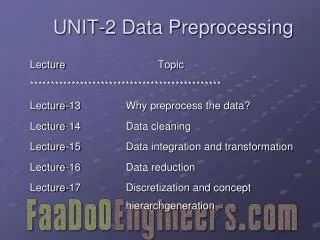
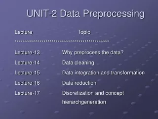
UNIT-II Data Preprocessing. Why preprocess the data?. Why Data Preprocessing?. Data in the real world is dirty incomplete : lacking attribute values, lacking certain attributes of interest, or containing only aggregate data noisy : containing errors or outliers

UNIT-II Data Preprocessing
E N D
Presentation Transcript
UNIT-IIData Preprocessing • Why preprocess the data?
Why Data Preprocessing? • Data in the real world is dirty • incomplete: lacking attribute values, lacking certain attributes of interest, or containing only aggregate data • noisy: containing errors or outliers • inconsistent: containing discrepancies in codes or names • No quality data, no quality mining results! • Quality decisions must be based on quality data • Data warehouse needs consistent integration of quality data
Multi-Dimensional Measure of Data Quality • A well-accepted multidimensional view: • Accuracy • Completeness • Consistency • Timeliness • Value added • Interpretability • Accessibility
Major Tasks in Data Preprocessing • Data cleaning • Data integration • Data transformation • Data reduction • Data discretization
Major Tasks in Data Preprocessing • Data cleaning • Fill in missing values, smooth noisy data, identify or remove outliers, and resolve inconsistencies • Data integration • Integration of multiple databases, data cubes, or files • Data transformation • Normalization and aggregation • Data reduction • Obtains reduced representation in volume but produces the same or similar analytical results • Data discretization • Part of data reduction but with particular importance, especially for numerical data
Data Cleaning • Data cleaning tasks • Fill in missing values • Identify outliers and smooth out noisy data • Correct inconsistent data
Missing Data • Data is not always available • E.g., many tuples have no recorded value for several attributes, such as customer income in sales data • Missing data may be due to • equipment malfunction • inconsistent with other recorded data and thus deleted • data not entered due to misunderstanding • certain data may not be considered important at the time of entry • not register history or changes of the data • Missing data may need to be inferred.
How to Handle Missing Data? • Ignore the tuple : usually done when class label is missing (assuming the tasks in classification—not effective when the percentage of missing values per attribute varies considerably. • Fill in the missing value manually • Use a global constant to fill in the missing value: e.g., “unknown”, a new class?! • Use the attribute mean to fill in the missing value • Use the attribute mean for all samples belonging to the same class to fill in the missing value • Use the most probable value to fill in the missing value: inference-based such as Bayesian formula or decision tree
Noisy Data • Noise: random error or variance in a measured variable • Incorrect attribute values may due to • faulty data collection instruments • data entry problems • data transmission problems • technology limitation • inconsistency in naming convention • Other data problems which requires data cleaning • duplicate records • incomplete data • inconsistent data
How to Handle Noisy Data? • Binning method: • first sort data and partition into (equi-depth) bins • then one can smooth by bin means, smooth by bin median, smooth by bin boundaries, etc. • Clustering • detect and remove outliers • Combined computer and human inspection • detect suspicious values and check by human • Regression • smooth by fitting the data into regression functions
Simple Discretization Methods: Binning • Equal-width (distance) partitioning: • It divides the range into N intervals of equal size: uniform grid • if A and B are the lowest and highest values of the attribute, the width of intervals will be: W = (B-A)/N. • Equal-depth (frequency) partitioning: • It divides the range into N intervals, each containing approximately same number of samples • Good data scaling • Managing categorical attributes can be tricky.
Data Smoothing Techniques * Sorted data for price (in dollars): 4, 8, 9, 15, 21, 21, 24, 25, 26, 28, 29, 34 * Partition into (equi-depth) bins: - Bin 1: 4, 8, 9, 15 - Bin 2: 21, 21, 24, 25 - Bin 3: 26, 28, 29, 34 * Smoothing by bin means: - Bin 1: 9, 9, 9, 9 - Bin 2: 23, 23, 23, 23 - Bin 3: 29, 29, 29, 29 * Smoothing by bin boundaries: - Bin 1: 4, 4, 4, 15 - Bin 2: 21, 21, 25, 25 - Bin 3: 26, 26, 26, 34
Inconsistent data • It occur due to • - error during data entry, functional dependencies b/w attributes and missing values • Detected and corrected by manually or knowledge engineering tools
Data Cleaning as a Process • Data discrepancy detection • - Rules & tools • Data transformation • - Tools 9/18/2014 17
Data discrepancy detection • First step in data cleaning process • Use metadata (e.g., domain, range, dependency, distribution) & rules to detect discrepancy • 1. Unique rule • 2. Consecutive rule and • 3. Null rule • Unique rule – each value of the given attribute is different from all other values for that attribute. • Consecutive rule – no missing values b/w lowest & highest value for that attribute • Null rule - specifies use of blanks ,?, special char or string indicates null value
Discrepancy detection tools • Data scrubbing tool • Data auditing tool • Data scrubbing: usesimple domain knowledge (e.g., postal code, spell-check) to detect errors and make corrections • Data auditing: by analyzing data to discover rules and relationship to detect violators (e.g., correlation and clustering to find outliers)
Data transformation • II step in data cleaning as a process • Need to define and apply transformation to correct them
Data transformation Tools • Data migration tools • ETL (Extraction/Transformation/Loading) tools • Data migration tools: allow transformations to be specified( eg.replace “ gender” by “sex” • ETL(Extraction/Transformation/Loading) tools:allow users to specify transformations through a graphical user interface
Data Integration • Data integration • combines data from multiple sources into a coherent store Issues • schema Integration and object matching • Redundancy • Detection and Resolution of data value conflict
Schema integration: • integrate metadata from different sources • [Univ (2 M)] Entity identification problem: • Same entity can be represented in different forms in different table. • Iidentify real world entities from multiple data sources, e.g., A.cust-id B.cust-# • Detecting and resolving data value conflicts • For the same real world entity, attribute values from different sources are different • possible reasons: different representations, different scales, e.g., metric vs. British units
Handling Redundant Data in Data Integration • Redundant data occur often when integration of multiple databases • The same attribute may have different names in different databases • One attribute may be a “derived” attribute in another table, e.g., annual revenue • Redundant data may be able to be detected by co-relational analysis • Careful integration of the data from multiple sources may help reduce/avoid redundancies and inconsistencies and improve mining speed and quality
Correlation Analysis (Numeric Data) Correlation coefficient (also called Pearson’s product moment coefficient) where n is the number of tuples, and are the respective means of p and q, σp and σq are the respective standard deviation of p and q, and Σ(pq) is the sum of the pq cross-product. If rp,q > 0, p and q are positively correlated (p’s values increase as q’s). The higher, the stronger correlation. rp,q = 0: independent( no correlation); rpq < 0: negatively correlated (p,q – attribute) 9/18/2014 26
Data Transformation • data are transformed or consolidate into form appropriate for mining. • It Involves, • smoothing • Aggregation • Generalization of the data • Normalization • Attribute Construction
Data Transformation • Smoothing:remove noise from data • Aggregation: summarization, data cube construction • Generalization: concept hierarchy climbing • Normalization: scaled to fall within a small, specified range( -1.0 to 1.0 or 0.0 to 1.0) • min-max normalization • z-score normalization • normalization by decimal scaling • Attribute/feature construction • New attributes constructed from the given ones
Data Transformation: Normalization • min-max normalization( perform linear transformation) • z-score normalization( or Zero mean normalization) • normalization by decimal scaling Where j is the smallest integer such that Max(| |)<1
min-max normalization • Pblm: suppose that the minimum and maximum values for the attribute income are $1,000 and $15,000 respectively. Map income to the range[0.0,1.0].By min-max normalization, a value of $12,000 for income is transformed to?
Ans: = 12000-1000/15000-1000(1.0-0)+0 = 0.785
z-score normalization • Suppose that the mean and standard deviation of the values for the attribute income are $52,000 and $14,000.with Z- score normalization, a value of $72,000 for income is transformed to ?
Ans: = 72000-52,000/14,000 = 1.42
Data Reduction Strategies • Warehouse may store terabytes of data: Complex data analysis/mining may take a very long time to run on the complete data set • Data reduction • Obtains a reduced representation of the data set that is much smaller in volume but yet produces the same (or almost the same) analytical results • Data reduction strategies • Data cube aggregation • Dimensionality reduction • Data Compression • Numerosity reduction(2m-univ) • Discretization and concept hierarchy generation
Numerosity reduction(2m-univ) • Data replaced by parametric model (store only parameters instead of data value) or non parametric model ( clustering, sampling ,..etc..)
Data Cube Aggregation • The lowest level of a data cube • the aggregated data for an individual entity of interest • Multiple levels of aggregation in data cubes • Further reduce the size of data • Reference appropriate levels • Use the smallest representation which is enough to solve the task • Queries regarding aggregated information should be answered using data cube, when possible
Dimensionality ReductionAttribute subset selection • Feature selection (Attribute selection): • Goal: Find a minimum set of attributesuch that the resulting probability distribution of data classes given the values for those features is as close as possible to the original distribution obtained using all attributes. • reduce # of attributes discovered in the patterns, easier to understand • The best & worst attribute is determined using a test of statistical significance • Classification information gain measure
How we can find a “good” subset of the original attributes? • D attribute-2d possible subset- exhaustive search expensive • Heuristic methods ( it will reduce search space-used for attribute subset selection): • step-wise forward selection • step-wise backward elimination • combining forward selection and backward elimination • decision-tree induction
Initial attribute set { A1,A2,A3,A4,A5,A6} • Forward Selection • {} • {A1} • {A1,A4] Reduced attribute set • {A1,A4,A6} • Backward elimination • { A1,A3,A4,A5,A6} • { A1,A4,A5,A6} Reduced attribute set • { A1,A4, A6}
> Example of Decision Tree Induction Initial attribute set: {A1, A2, A3, A4, A5, A6} A4 ? A6? A1? Class 2 Class 2 Class 1 Class 1 Reduced attribute set: {A1, A4, A6}
Dimensionality Reduction • Data Compression • String compression • There are extensive theories and well-tuned algorithms • Typically lossless • But only limited manipulation is possible without expansion • Audio/video compression • Typically lossy compression, with progressive refinement • Sometimes small fragments of signal can be reconstructed without reconstructing the whole • Time sequence is not audio • Typically short and vary slowly with time
Data Compression Original Data Compressed Data lossless Original Data Approximated lossy
Haar2 Daubechie4 Wavelet Transforms • Discrete wavelet transform (DWT): linear signal processing • Compressed approximation: store only a small fraction of the strongest of the wavelet coefficients • Similar to discrete Fourier transform (DFT), but better lossy compression, localized in space • Method: • Length, L, must be an integer power of 2 (padding with 0s, when necessary) • Each transform has 2 functions: smoothing, difference • Applies to pairs of data, resulting in two set of data of length L/2 • Applies two functions recursively, until reaches the desired length
Principal Component Analysis • Given N data vectors from k-dimensions, find c <= k orthogonal vectors that can be best used to represent data • The original data set is reduced to one consisting of N data vectors on c principal components (reduced dimensions) • Each data vector is a linear combination of the c principal component vectors • Works for numeric data only • Used when the number of dimensions is large
Principal Component Analysis X2 Y1 Y2 X1
Numerosity Reduction • Parametric methods • Assume the data fits some model, estimate model parameters, store only the parameters, and discard the data (except possible outliers) • Log-linear models: obtain value at a point in m-D space as the product on appropriate marginal subspaces • Non-parametric methods • Do not assume models • Major families: histograms, clustering, sampling
Regression and Log-Linear Models • Linear regression: Data are modeled to fit a straight line • Often uses the least-square method to fit the line • Multiple regression: allows a response variable Y to be modeled as a linear function of multidimensional feature vector • Log-linear model: approximates discrete multidimensional probability distributions
Regress Analysis and Log-Linear Models • Linear regression: Y = + X • Two parameters , and specify the line and are to be estimated by using the data at hand. • using the least squares criterion to the known values of Y1, Y2, …, X1, X2, …. • Multiple regression: Y = b0 + b1 X1 + b2 X2. • Many nonlinear functions can be transformed into the above. • Log-linear models: • The multi-way table of joint probabilities is approximated by a product of lower-order tables. • Probability: p(a, b, c, d) = ab acad bcd
Histograms • A popular data reduction technique • Divide data into buckets and store average (sum) for each bucket • Can be constructed optimally in one dimension using dynamic programming • Related to quantization problems.