Download
1 / 2
30 likes | 115 Views
Explore the efficient control and trajectory optimization of an occulter-based exoplanet-finding telescope to enhance imaging of stars and planets. Learn about the formation flying of occulters and optimal configurations for maximum sky coverage.

E N D
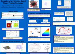
Dynamics of an Occulter Based Planet Finding Telescope C E A D F B Operating range Egemen Kolemen, N. Jeremy Kasdin Dept. of Mechanical and Aerospace Eng., Princeton University Due to reflection of sunlight from the occulter Including the constraint of the formation not being able to look towards or away from the Sun direction, we get a time dependent ordering problem as shown on the right. Finding Quasi-Halos: A fast, robust, fully numeric method employing multiple Poincare sections to find the quasi-periodic orbits around libration points is developed along with a numerical method to transport the R3BP results to the full ephemeris model. Relative motion between a Quasi-Halo and a Halo in the inertial frame. Further Optimization with best TSP outputs 1. Mission Basics 3. Trajectory Optimization and Control Once done choose the best ~1000 solutions and go to SQP for fine tuning (we averaged and didn’t use the full ephemeris) and more importantly optimizing the time between each imaging session Need for control: Fuel-free Quasi-Halo trajectories are very suitable to place the occulter but they are too slow to image the required number of stars in the approximate 5 year life time without control. Two approaches: 1. Multiple occulters employing the fuel-free trajectories. 2. Single occulter with minimal-fuel consumption trajectory. Occulter Telescope a. Single Occulter Optimization Formation flying of an occulter is proposed to enhance the optical performance of an exo-planet imaging telescope. • ) Further Optimization with best TSP outputs Hh J j Optimal Control of the occulter between two imaging sessions can be converted into a two-point boundary value problem (TPBVP) with algebraic constraints via Euler-Lagrange Formulation. Under simplifying assumptions Hu can be solved for and the problem is converted to a convex TPBVP. A very fast implementation of this algorithm enables finding the optimal trajectories as a function of the significant parameters. b. Multiple Occulter Optimization The contrast between the planet and the target star is reduced by suppressing most of the light from the target star before it enters the optical system. The occulter shape is optimized such that the intensity of light from the star is minimal in the possible planet locations on the image plane. Multiple occulters using the fuel free Quasi-Halo Trajectories 2 multiple s/c Figure – multiple s/c in the skyplot 3 parameters per s/c that define the unique quasi-halo and position on it x number of s/c = total variables Using the fast quasi-halo generation; Find the best configuration for the most sky coverage by optimizing the above parameters Fine tune to find the orbits that come close to the given star set (Assume no control); This gives you the ball part of the solution; Combine both – find the minimum fuel maximum imaging space of variables Optimization in stages: 1. Maximize total sky coverage, obtain the region of parameters 2. Maximize target star coverage within Stage 1 solutions • • (degrees) • The formation is proposed to be around a Halo orbit near the L2 point of the Earth-Sun system. Reasons: • 1. Far away from Earth to avoid interference. • 2. Good telecommunication properties. • 3. Minimal fuel is needed to get to and station keep the orbits. Left: The sphere of possible occulter locations about the telescope at two times and example optimal trajectories connecting them. Right: Surface of optimal Delta-V's as a function of distance from the telescope and angle between the LOS vectors of consecutively imaged star (Averaged over millions of simulations). 2. Dynamics around the Libration Point Time Dependent Dynamical Traveling Salesman Problem References 1. E. Kolemen & N. J. Kasdin, “Optimal Trajectory Control of an Occulter Based Planet Finding Telescope”, To be presented at the AAS Guidance & Control Conference, Breckenridge, Colorado, AAS 07-036, Feb. 2007. 2. E. Kolemen & N. J. Kasdin, “Optimal Configuration of a Planet-Finding Mission Consisting of a Telescope and a Constellation of Occulters”, To be presented at the AAS/AIAA Space Flight Mechanics Meeting, Sedona, Arizona, AAS 07-202, Jan. 2007. 3. E. Kolemen, N. J. Kasdin & P. Gurfil, “Quasi-Periodic Orbits of the Restricted Three Body Problem Made Easy”, Proceedings of the New Trends in Astrodynamics and Applications, Aug. 2006 4. W. Cash, “Detection of Earth-like planets around nearby stars using a petal shaped occulter”, Nature, 442, 51-53, 6 July 2006. 5. J. Arenberg, A. Lo, C. Lillie, R. Malmstrom, R. Polidan, C. Noecker & W. Cash, “Occulter Systems Terrestrial Planet Finding”, Terrestrial Planet Finder Coronagraph Workshop, Pasadena, CA, Sep. 28-29, 2006. An example sequence of star imaging on the skyplot and the Branch-And-Cut Algorithm for solving TSP. Periodic phase-space around L2 shown in 3D and on a Poincare section.
What the mission is • Explain the optical system • L2 and mission formation • Dynamics around L2 • Talk about new method to find the quasi-periodic orbits and how to move them to JPL-406 • Quasi-Halos – why they are good • 2 options since quasi-halos are slow • 1 s/c find the minimum fuel consumption • Optimization between 2 star imaging session. • Figure – example trajectories • Problem statement • Simplified E-L equations • Figure - After 20 million simulations and averaging • TSMP • Figure – Tree • Figure – Constraint and the matrix (traveling salesman) • Talk about time dependent – dynamics TSMP • Fine tune and optimize time between imaging sessions • Once done choose the best ~1000 solutions and go to SQP for fine tuning (we averaged and didn’t use the full ephemeris) and more importantly optimizing the time between each imaging session • SQP equation • Figure – SQP with time optimization • 2 multiple s/c • Figure – multiple s/c in the skyplot • 3 parameters per s/c that define the unique quasi-halo and position on it x number of s/c = total variables • Using the fast quasi-halo generation; Find the best configuration for the most sky coverage • Fine tune to find the orbits that come close to the given star set (Assume no control); This gives you the ball part of the solution; • Combine both – find the minimum fuel maximum imaging space of variables