Download
1 / 17
190 likes | 500 Views
Seminar on MEASURES OF DISPERSION. Presented by JAYAKUMARA Research Scholar. INTRODUCTION.

E N D
Seminar onMEASURES OF DISPERSION Presented by JAYAKUMARA Research Scholar
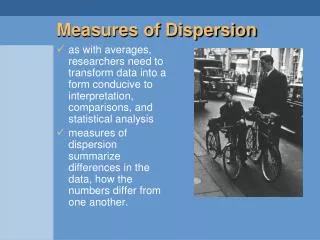
INTRODUCTION • The Measures of central tendency gives us a birds eye view of the entire data they are called averages of the first order, it serve to locate the centre of the distribution but they do not reveal how the items are spread out on either side of the central value. The measure of the scattering of items in a distribution about the average is called dispersion.
INTRODUCTION • Dispersion measures the extent to which the items vary from some central value. It may be noted that the measures of dispersion or variation measure only the degree but not the direction of the variation. The measures of dispersion are also called averages of the second order because they are based on the deviations of the different values from the mean or other measures of central tendency which are called averages of the first order.
DEFINITION • In the words of Bowley “Dispersion is the measure of the variation of the items” According to Conar “Dispersion is a measure of the extent to which the individual items vary”
METHODS OF MEASURING DISPERSION • Range • Quartile Deviation • Mean Deviation • Standard Deviation
RANGE • It is defined as the difference between the smallest and the largest observations in a given set of data. • Formula is R = L – S • Ex. Find out the range of the given distribution: 1, 3, 5, 9, 11 • The range is 11 – 1 = 10.
QUARTILE DEVIATION • It is the second measure of dispersion, no doubt improved version over the range. It is based on the quartiles so while calculating this may require upper quartile (Q3) and lower quartile (Q1) and then is divided by 2. Hence it is half of the deference between two quartiles it is also a semi inter quartile range. The formula of Quartile Deviation is • (Q D) = Q3 - Q1 2
MEAN DEVIATION • Mean Deviation is also known as average deviation. In this case deviation taken from any average especially Mean, Median or Mode. While taking deviation we have to ignore negative items and consider all of them as positive. The formula is given below
MEAN DEVIATION The formula of MD is given below MD = d N (deviation taken from mean) MD = m N (deviation taken from median) MD = z N (deviation taken from mode)
STANDARD DEVIATION • The concept of standard deviation was first introduced by Karl Pearson in 1893. The standard deviation is the most useful and the most popular measure of dispersion. Just as the arithmetic mean is the most of all the averages, the standard deviation is the best of all measures of dispersion.
STANDARD DEVIATION • The standard deviation is represented by the Greek letter (sigma). It is always calculated from the arithmetic mean, median and mode is not considered. While looking at the earlier measures of dispersion all of them suffer from one or the other demerit i.e. • Range –it suffer from a serious drawback considers only 2 values and neglects all the other values of the series.
STANDARD DEVIATION • Quartile deviation considers only 50% of the item and ignores the other 50% of items in the series. • Mean deviation no doubt an improved measure but ignores negative signs without any basis. • Karl Pearson after observing all these things has given us a more scientific formula for calculating or measuring dispersion. While calculating SD we take deviations of individual observations from their AM and then each squares. The sum of the squares is divided by the number of observations. The square root of this sum is knows as standard deviation.
MERITS OF STANDARD DEVIATION • Very popular scientific measure of dispersion • From SD we can calculate Skewness, Correlation etc • It considers all the items of the series • The squaring of deviations make them positive and the difficulty about algebraic signs which was expressed in case of mean deviation is not found here.
DEMERITS OF STANDARD DEVIATION • Calculation is difficult not as easier as Range and QD • It always depends on AM • Extreme items gain great importance The formula of SD is = √∑d2 N Problem: Calculate Standard Deviation of the following series X – 40, 44, 54, 60, 62, 64, 70, 80, 90, 96
Standard deviation • AM = X N • = 660 = 66 AM • 10 SD = √∑d2 N • SD =√3048 = 17.46 • 10
Bibliography • Sony, R.S.(2009). Essential business mathematics and statistics. New Delhi: Ane books. Thank you