MEASURES OF DISPERSION

1. MEASURES OF DISPERSION

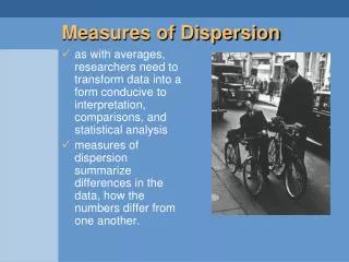
2. The measures of central tendency, such as the mean, median and mode, do not reveal the whole picture of the distribution of a data set. Two data sets with the same mean may have completely different spreads. The variation among the values of observations for one data set may be much larger or smaller than for the other data set. NOTE: the words dispersion, spread and variation have the same meaning. MEASURES OF DISPERSION

3. Consider the following two data sets on the ages of all workers in each of two small companies. Company 1: 47 38 35 40 36 45 39 Company 2: 70 33 18 52 27 The mean age of workers in both these companies is the same: 40 years. By knowing only these means, we may deduce that the workers have a similar age distribution in the two companies. But, the variation in the workers’ age is very different for each of these two companies. MEASURES OF DISPERSION: example Company1 36 39 35 38 40 45 47 It has a much larger variation than ages of the workers in the first company Company2 18 27 33 52 70

4. The mean, median or mode is usually not by itself a sufficient measure to reveal the shape of a distribution of a data set. We also need a measure that can provide some information about the variation among data set values. • The measures that help us to know about the spread of adata set are called measures of dispersion. • The measures of central tendency and dispersion taken together give a better picture of a data set. • We consider 3 measures of dispersion: • Range • Variance • Standard Deviation MEASURES OF DISPERSION

5. Definition the range is the simplest measure of dispersion and it is obtained by taking the difference between the largest and the smallest values in a data set: RANGE = LARGEST VALUE – SMALLEST VALUE RANGE

6. The following data set gives the total areas in square miles of the 4 western South-Central statesof the United States. RANGE: example RANGE = LARGEST VALUE – SMALLEST VALUE = 267,277 – 49,651 = 217,626 square miles Thus, the total areas of these four states are spread over a range of 217,626 square miles.

7. The range, like the mean has the disadvantage of being influenced by outliers. Consequently, it is not a good measure of dispersion to use for data set containing outliers. • The calculation of the range is based on two values only: the largest and the smallest. All other values in a data set are ignored. • Thus, the range is not a very satisfactory measure of dispersion and it is, in fact, rarely used. RANGE: disadvantages

8. Definition Thevarianceis a measure of dispersion of values based on their deviation from the mean. The variance is defined to be: for a population VARIANCE for a sample

9. The difference between an observation and the mean, ( or ) is called dispersion from the mean. Consequently, the variance can also be defined as the arithmetic mean of the squared deviationsfrom the mean. From the computational point of view, it is easier and more efficient to use short-cut formulas to calculate the variance VARIANCE

10. Refer to the data on 2002 total payrolls of 5 Major League Baseball (MLB) teams. VARIANCE: example 1

11. We apply the short-cut formula, hence we need to compute the squares of observations x2. VARIANCE: example 1

12. The following data are the 2002 earnings (in thousands of dollars) before taxes for all 6 employees of a small company. 48.50 38.40 65.50 22.60 79.80 54.60 VARIANCE: example 2

13. The formula for variance changes slightly if observations are grouped into a frequency table. Squared deviations are multiplied by each frequency's value, and then the total of these results is calculated. for a population for a sample VARIANCE: frequency distribution The short-cut formulas become:

14. VARIANCE: example 3

15. Variance: frequency distribution with classes Again, when the data set is organized in a frequency distribution with classes, we are approximating the data set by "rounding" each value in a given class to the class midpoint. Thus, the variance of a frequency distribution is given by Short-cut formulas for a population for a sample where mi is the midpoint of each class interval.

16. Variance:example 4 The following table gives the frequency distribution of the number of orders received each day during the past 50 days at the office of a mail-order company.

17. Definition The standard deviation is the positive square root of the variance. for a population STANDARD DEVIATION for a sample

18. STANDARD DEVIATION The standard deviation is the most used measure of dispersion. The value of the standard deviation tells how closely the values of a data set are clustered around the mean. In general, a lower value of the standard deviation for a data set indicates that the values of that data set are spread over a relatively smaller range around the mean. In contrast, a large value of the standard deviation for a data set indicates that the values of that data set are spread over a relatively large range around the mean.

19. STANDARD DEVIATION: example 1

20. STANDARD DEVIATION: example 2

21. The values of the variance and the standard deviation are never negative. That is, the numerator in the formula for the variance should never produce a negative value. Usually the values of the variance and standard deviation are positive, but if data set has no variation, then the variance and standard deviation are both zero. Example: 4 persons in a group are the same age – say 35 years. If we calculate the variance and the standard deviation, their values are zero. Variance and Standard Deviation: observations

22. CONTINGENCY TABLES AND ELEMENTS OF PROBABILITY

23. CONTINGENCY TABLES The variables are usually presented as a contingency table (or two-way classification table). In manyapplications the interest isfocused on the joint analysisoftwovariables (qualitative and/or quantitative) with the aimofevaluating the relation betweenthem. Whereas a frequency distribution provides the distribution of one variable, a contingency table describes the distribution of two or more variables simultaneously.

24. All 420 employeesof a company wereaskedifthey are smokers or nonsmokers and whether or notthey are college graduates. CONTINGENCY TABLES Joint frequency of category “Smoker” of X and “Not a college Graduate” of Y Cell The table gives the distribution of 420 employees based on two variables or characters: X-smoke (yes or not) and Y-graduation (yes or not)

25. CONTINGENCY TABLES: marginal distributions Marginal distribution X Y X Marginal distribution Y Grand Total The right-hand column and the bottom row are called marginal distribution of X and marginal distribution of Y respectively.

26. CONTINGENCY TABLES Marginal distribution Y Marginal distribution X X Y

27. CONTINGENCY TABLES: conditional distributions Conditional distribution of X to the category “College Graduate” of Y Conditionaldistributionof Y to the category “Smoker” of X Y X X Y NOTE

28. Definition of probability There are threedifferentdefinitionsofprobability: classicaldefinitionofprobability, frequentistdefinitionofprobability, subjective (Bayesian) definitionofprobability. Frequentistdefinitionofprobability: The relative frequencyassociatedto a categoryof a variable (event) analyzed can beinterpretedasanapproximationof the probabilityassociatedtothatevent.

29. Definition of probability Example: Ten of the 500 randomly selected cars manufactured at a certain auto factory are found to be lemons. Assuming that the lemons are manufactured randomly, what is the probability that the next car manufactured at this auto factory is a lemon? NOTE:The relative frequencyisanapproximationof the probability!! Relative frequencies and probabilitiesgetcloseras the numberofcarsincreases.

30. Marginal Probability Coming back to the exampleof the 420 employees. Suppose thatoneemployeeisselected at randomfrom the 420 employees. Hemaybeclassified on the basisofsmoke alone or graduation. The employee can be “smoker”, “nonsmoker”, “graduate”, “nongraduate”. The probabilityofeachcharacteristiciscalledmarginalprobability

31. Marginal Probability Marginal (Simple) Probability: is the probability (relative frequency) computed on the marginal distributions:

32. Joint Probability Suppose that one employees is selected at random from these 420. What is the probability that the employee is a smoker and a College graduate? It is written asP (Smoker College Graduate). The symbol  is read as “and”.

33. Joint Probability JointProbability: isthe probability (relative frequency) computed on the joint distributions

34. Conditional Probability Now suppose that one employees is selected at random from these 420. Assume that it is known that he is a Smoker. What is the probability that the employee selected is Graduate? It is written asP (Graduate|Smoker) It is read as “Probability that he is College Graduate given that he is a Smoker”

35. Conditional Probability Conditional Probability: is the probability (relative frequency) computed on the conditional distributions: