Download
1 / 52
1.21k likes | 2.51k Views
ANOVA One-Way and Two-way Analyses of Variance. PSBE Chapters 14, 15 and Guan Chapter 9. Research Questions. Income and allocation? Do people in different counties earn same income? Obviously it is not, how can we test?. Research Questions. Income and gender?

E N D
ANOVA One-Way and Two-way Analyses of Variance PSBE Chapters 14, 15 and Guan Chapter 9
Research Questions • Income and allocation? • Do people in different counties earn same income? • Obviously it is not, how can we test?
Research Questions • Income and gender? • Do men and women earn same income? • Do industrial and service industries offer same salary • Obviously it is not, how can we test?
The idea of ANOVA (變異數分析) A factor (因子) is a variable that can take one of several levels used to differentiate one group from another. An experiment has a one-way or completely randomized design (完全隨機設計) if several levels of one factor are being studied and the individuals are randomly assigned to its levels. (There is only one way to group the data.) • Example: Which of four advertising offers mailed to sample households produces the highest sales? • Will a lower price in a plain mailing draw more sales on average than a higher price in a fancy brochure? Analyzing the effect of price and layout together requires two-way ANOVA. Analysis of variance (ANOVA) is the technique used to determine whether more than two population means are equal. One-way ANOVA is used for completely randomized, one-way designs.
The ANOVA setting: comparing means We want to know if the observed differences in sample means are likely to have occurred by chance just because of the random sampling. This will likely depend on both the difference between the sample means and how much variability there is within each sample.
The two-sample t statistic A two sample t test assuming equal variance and an ANOVA comparing only two groups will give you the exact same p-value (for a two-sided hypothesis). H0: m1=m2 Ha: m1≠m2 t test assuming equal variance t statistic H0: m1=m2 Ha: m1≠m2 One-way ANOVA F-statistic F = t2 and both p-values are the same. But the t test is more flexible: You may choose a one-sided alternative instead, or you may want to run a t test assuming unequal variance if you are not sure that your two populations have the same standard deviation s.
The ANOVA model Random sampling always produces chance variations. Any “factor effect” would thus show up in our data as the factor-driven differences plus chance variations (“error”): Data = fit (“factor/groups”) + residual (“error”) The one-way ANOVA model analyses situations where chance variations are normally distributed N(0,σ) so that:
Testing hypotheses in one-way ANOVA We have I independent SRSs, from I populations or treatments. The ith population has a normal distribution with unknown mean µi. All I populations have the same standard deviation σ, unknown. The ANOVA F statistic tests: H0: m1 = m2 = … = mI Ha: not all the mi are equal When H0 is true, F has the F distributionwith I − 1 (numerator) and N − I (denominator) degrees of freedom.
The ANOVA F-test TheANOVA F-statisticcompares variation due to specific sources (levels of the factor) to variation among individuals who should be similar (individuals in the same sample). Difference in means large relative to overall variability Difference in means small relative to overall variability F tends to be small F tends to be large Larger F-values typically yield more significant results. How large depends on the degrees of freedom (I− 1 and N − I).
Checking our assumptions The ANOVA F-test requires that all populations have thesame standard deviation s. Since s is unknown, this can be hard to check. Each of the #I populations must be normally distributed (histograms or normal quantile plots). But the test is robust to normality deviations for large enough sample sizes, thanks to the central limit theorem. Practically: The results of the ANOVA F-test are approximately correct when the largest sample standard deviation is no more than twice as large as the smallest sample standard deviation. (Equal sample sizes also make ANOVA more robust to deviations from the equal σ rule)
The ANOVA table R2 = SSG/SST √MSE = sp Coefficient of determination Pooled standard deviation The sum of squares represents variation in the data: SST = SSG + SSE. The degrees of freedom likewise reflect the ANOVA model: DFT = DFG + DFE. Data (“Total”) = fit (“Groups”) + residual (“Error”)
Case: Do eyes affect ad response? • A study investigated the affect of the color of a model’s eyes in a viewer’s response to an ad. In three groups of students, viewers see a picture of the model looking directly at the camera, with only the eye color being changed. A fourth group of students saw a picture of the model looking down. • The table below summarizes the responses :
Verifying conditions for ANOVA Side-by-side boxplots of the scores for the four groups. The data appear relatively symmetric with some skewness.
Verifying conditions for ANOVA Normal quantile plots of the scores for the four groups. The data looks reasonably Normal.
ANOVA results The pooled standard deviation sp is reported as 1.677. The value of F is 2.89, with a P-value of 0.036. We have evidence at the 5% significance level to reject the null hypotheses that the four populations have equal means. There is evidence that the four groups of students do not all have the same mean attitude score.
Using Table E The F distribution is asymmetrical and has two distinct degrees of freedom. This was discovered by Fisher, hence the label “F.” Once again, what we do is calculate the value of F for our sample data and then look up the corresponding area under the curve in Table E.
Yogurt preparation and taste Yogurt can be made using three distinct commercial preparation methods: traditional, ultra filtration, and reverse osmosis. To study the effect of these methods on taste, an experiment was designed in which three batches of yogurt were prepared for each of the three methods. A trained expert tasted each of the nine samples (presented in random order), and judged them on a scale of 1 to 10. Variables, hypotheses, assumptions, calculations?
dfnum = I− 1 F dfden=N−I
Computation details MSG, the mean square for groups, measures how different the individual means are from the overall mean (~ weighted average of square distances of sample averages to the overall mean). SSG is the sum of squares for groups. MSE, the mean square for error, is the pooled sample variance sp2 and estimates the common variance σ2of the I populations (~ weighted average of the variances from each of the I samples). SSE is the sum of squares for error.
One-Way ANOVA Comparing Group Means and the Power of the ANOVA Test
You have calculated a p-value for your ANOVA test. Now what? If you found a significant result, you still need to determine which treatments were different from which. • You can gain insight by looking back at your plots (boxplot, mean ± s). • There are several tests of statistical significance designed specifically for multiple tests. You can choose, apriori,contrasts or, aposteriori,multiple comparisons. • You can find the confidence interval for each mean mi shown to be significantly different from the others.
Contrasts can be used only when there are clear expectations BEFORE starting an experiment, and these are reflected in the experimental design. Contrasts are planned comparisons. • Patients are given either drug A, drug B, or a placebo. The three treatments are not symmetrical. The placebo is meant to provide a baseline against which the other drugs can be compared. • Multiple comparisons should be used when there are no justified expectations. Those are aposteriori, pair-wise tests of significance. • We compare gas mileage for eight brands of SUVs. We have no prior knowledge to expect any brand to perform differently from the rest. Pair-wise comparisons should be performed here, but only if an ANOVA test on all eight brands reached statistical significance first. It is NOT appropriate to use a contrast test when suggested comparisons appear only after the data is collected.
Contrasts: planned comparisons When an experiment is designed to test a specific hypothesis that some treatments are different from other treatments, we can use contrasts to test for significant differences between these specific treatments. • Contrasts are more powerful than multiple comparisons because they are more specific. They are better able to pick up a significant difference. • You can use a t test on the contrasts or calculate a t confidence interval. • The results are valid regardless of the results of your multiple sample ANOVA test (you are still testing a valid hypothesis).
To test the null hypothesis H0: y = 0 use the t statistic: with degrees of freedom DFE that is associated with sp. The alternative hypothesis can be one or two sided. A contrast is a combination of population means of the form: where the coefficients ai have sum 0. The corresponding sample contrast is : The standard error of c is: A level C confidence interval for the difference y is: where t* is the critical value defining the middle C% of the t distribution with DFE degrees of freedom.
Contrasts are not always readily available in statistical software packages (when they are, you need to assign the coefficients “ai”), or they may be limited to comparing each sample to a control. If your software doesn’t provide an option for contrasts, you can test your contrast hypothesis with a regular t test using the formulas we just highlighted. Remember to use the pooled variance and degrees of freedom as they reflect your better estimate of the population variance. Then you can look up your p-value in a table of t distribution. [SAS code] proc glm data = ….; class b; model y = b; means b /deponly; contrast 'Compare 3rd & 4th grp' b 0 0 1 -1; contrast 'Compare 1st & 2nd with 3rd & 4th grp' b 1 1 -1 -1; contrast 'Compare 1st, 2nd & 3rd grps with 4th grp' b 1 1 1 -3; run; quit;
Evaluation of the new product A study compares the reading comprehension (“COMP,” a test score) of children randomly assigned to one of three teaching methods: basal, DRTA, and strategies. We test: H0: µBasal = µDRTA = µStrat vs. Ha: H0 not true The ANOVA test is significant (α = 5%): we have found evidence that the three methods do not all yield the same population mean reading comprehension score.
Evaluation of the new product (cont.) • The two new methods are based on the same idea. Are they superior to the standard method? We can formulate this question as: H01: ½(µDRTA + µStrat)=µBasal vs. Ha1: ½(µDRTA + µStrat)>µBasal • Are the DRTA and Strat methods equally effective? We formulate this as: H02: µDRTA = µStrat vs. Ha2: µDRTA≠µStrat
Evaluation of the new product (cont.) • Output for contrasts for the comprehension scores in the new-product evaluation study: • The P-values are correct for two-sided alternative hypothesis. To convert the results to apply to our one-sided alternative Ha1, simply divide the reported P-value by two after checking that the sample contrast is positive. • There is strong evidence against H01, i.e., the new methods produce higher mean scores. However, there is not sufficient evidence against H02, i.e., the DRTA and Strat methods appear equally effective.
Multiple comparisons* Multiple comparison tests are variants on the two-sample t test. • They use the pooled standard deviation sp = √MSE. • The pooled degrees of freedom DFE. • And they compensate for the multiple comparisons. We compute the t statistic for all pairs of means: A given test is significant (µi and µj significantly different), when |tij| ≥ t** (df = DFE). The value of t** depends on which procedure you choose to use.
The Bonferroni procedure* The Bonferroni procedure performs a number of pair-wise comparisons with t tests and then multiplies each p-value by the number of comparisons made. This ensures that the probability of making any false rejection among all comparisons made is no greater than the chosen significance level α. As a consequence, the higher the number of pair-wise comparisons you make, the more difficult it will be to show statistical significance for each test. But the chance of committing a type I error also increases with the number of tests made. The Bonferroni procedure lowers the working significance level of each test to compensate for the increased chance of type I errors among all tests performed.
Simultaneous confidence intervals* We can also calculate simultaneous level C confidence intervals for all pair-wise differences (µi − µj)between population means: • spis the pooled variance, MSE. • t** is the t critical with degrees of freedom DFE = N – I, adjusted for multiple, simultaneous comparisons (e.g., Bonferroni procedure).
What do you conclude? The three methods do not yield the same results: We found evidence of a significant difference between DRTA and basal methods (DRTA gave better results on average), but the data gathered does not support the claim of a difference between the other methods (DRTA vs. strategies or basal vs. strategies).
Power* The power, or sensitivity, of a one-way ANOVA is the probability that the test will be able to detect a difference among the groups (i.e., reach statistical significance) when there really is a difference. Estimate the power of your test while designing your experiment to select sample sizes appropriate to detect an amount of difference between means that you deem important. • Too small a sample is a waste of experiment, but too large a sample is also a waste of resources. • A power of at least 80% is often suggested.
Power computations* ANOVA power is affected by: • the significance level a • the sample sizes and number of groups being compared • the differences between group means µi • the guessed population standard deviation You need to decide what alternative Ha you would consider important to detect statistically for the means µi and to guess the common standard deviation σ (from similar studies or preliminary work). The power computations then require calculating a noncentrality parameter λ, which follows the F distribution with DFG and DFE degrees of freedom to arrive at the power of the test.
Two-way ANOVAThe Two-Way ANOVA Model and Inference for Two-Way ANOVA
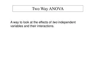
Two-way designs In a two-way design, two factors (independent variables) are studied in conjunction with the response (dependent) variable. Thus, there are two ways of organizing the data, as shown in a two-way table: two-way table (3 by 4 design to test the design of a magazine) When the dependent variable is quantitative, the data is analyzed with a two-way ANOVA procedure. A chi-square test is used instead if the dependent variable is categorical.
Advantages of a two-way ANOVA model • It is more efficient to study two factors at once than separately. A two-way design requires smaller sample sizes per condition than a series of one-way designs would, because the samples for all levels of factor B contribute to sampling for factor A. • Including a second factor thought to influence the response variable helps reduce the residual variation in a model of the data. In a one-way ANOVA for factor A, any effect of factor B is assigned to the residual (“error” term). In a two-way ANOVA, both factors contribute to the fit part of the model. • Interactions between factors can be investigated. The two-way ANOVA breaks down the fit part of the model between each of the main components (the two factors) and an interaction effect. The interaction cannot be tested with a series of one-way ANOVAs.
Interaction Two variables interact if a particular combination of variables leads to results that would not be anticipated on the basis of the main effects of those variables. • People of white descent have a higher per capita income than those of Asian descent. People from the Northeast have a higher per capita income than those from the Midwest. These are main effects.
Interaction An interaction implies that the effect of one variable differs depending on the level of another variable. • The ethnicity earnings gap is different in the two regions, so ethnicity and region interact.
Interaction An interaction implies that the effect of one variable differs depending on the level of another variable. Plot of per capita incomes of whites and Asians in two U.S. regions The main effect is seen in the different lines. Interaction is shown by the lack of parallelism.
Interaction An interaction implies that the effect of one variable differs depending on the level of another variable. Plot of per capita incomes of whites and Asians in two U.S. regions The main effect is seen in the different lines. Lack of interaction is shown by the parallel lines.
The two-way ANOVA model • We record a quantitative variable in a two-way design with I levels of the first factor and J levels of the second factor. • We have independent SRSs from each of I J Normal populations. Sample sizes do not have to be identical (although many software only carry out the computations when sample sizes are equal “balanced design”). • All parameters are unknown. The population means may be different but all populations have the same standard deviation σ.
Main effects and interaction effect • Each factor is represented by a main effect: this is the impact on the response (dependent variable) of varying levels of that factor, regardless of the other factor (i.e., pooling together the levels of the other factor). There are two main effects, one for each factor. • The interaction of both factors is also studied and is described by the interaction effect. • When there is no clear interaction, the main effects are enough to describe the data. In the presence of interaction, the main effects could mask what is really going on with the data.
Dependent var. Levels of factor A Levels of factor A Dependent var. B1 Levels of factor B: B2 Levels of factor A Levels of factor A Major types of two-way ANOVA outcomes In a two-way design, statistical significance can be found for each factor, for the interaction effect, or for any combination of these.
Inference for two-way ANOVA • A one-way ANOVA tests the following model of your data: Data (“total”) = fit (“groups”) + residual (“error”) So that the sum of squares and degrees of freedom are: SST = SSG + SSE DFT = DFG + DFE • A two-way design breaks down the “fit” part of the model into more specific subcomponents, so that: SST = SSA + SSB + SSAB + SSE DFT = DFA + DFB + DFAB + DFE Where A and B are the two main effects from each of the two factors, and AB represents the interaction of factors A and B.
The two-way ANOVA table • Main effects:P-value for factor A, P-value for factor B. • Interaction:P-value for the interaction effect of A and B. • Error:It represents the variability in the measurements within the groups. MSE is an unbiased estimate of the population variance s2.
Example: Discounts and expected prices • Does the frequency with which a supermarket product is offered at a discount affect the price that customers expect to pay for the product? Does the percent reduction also affect this expectation? We examine the data for two levels of promotion (1 and 3) and two levels of discount (40% and 20%). Thus, we have a two-way ANOVA with each factor having two levels, and 10 observations in each of the four treatment combinations. When promotions are increased from 1 to 3, expected price drops from $4.56 to $4.40. When the discount is increased from 20% to 40%, expected price drops from $4.61 to $4.35.