Population Genetics
640 likes | 1.06k Views
Population Genetics. The Hardy-Weinberg Law of Genetic Equilibrium In 1908 G. Hardy and W. Weinberg independently proposed that the frequency of alleles and genotypes in a population will remain constant from generation to generation if the population is stable and in genetic equilibrium.

Population Genetics
E N D
Presentation Transcript
Population Genetics The Hardy-Weinberg Law of Genetic Equilibrium In 1908 G. Hardy and W. Weinberg independently proposed that the frequency of alleles and genotypes in a population will remain constant from generation to generation if the population is stable and in genetic equilibrium.
Five conditions are required in order for a population to remain at Hardy-Weinberg Equilibrium: 1. A large breeding population 2. Random mating 3. No change in allelic frequency due to mutations 4. No immigration or emigration 5. No natural selection
If "A" and "a" are alleles for a particular gene and each diploid individual in a population has two such alleles, then p can be designated as the frequency of the "A" allele and q as the frequency of the "a" allele. Therefore, in a population of 100 individuals in which 40% of the genes are "A", p = 0.40. The rest of the genes (60%) would be "a", so q = 0.60.
This gives us Hardy-Weinberg's first equation: p + q = 1 In this example, 0.40 + 0.60 = 1.00. These values are referred to as allele frequencies.
As long as certain conditions are met, the frequency of the various combinations of these alleles (AA, Aa, aa) can be determined by using the second Hardy-Weinberg equation: p2 + 2pq + q2 = 1 • p2is the percentage of homozygous dominant individuals in the population • 2pq is the percentage of heterozygous individuals in the population and • q2 is the percentage of homozygous recessive individuals in the population.
Determining the Genotype and Allele Frequencies in a Population
Hardy-Weinberg Principle Hardy-Weinberg Equation
Using a Punnett Square for Hardy Weinberg Frequencies Example: The frequency of the T allele is 0.70. What is the frequency of the t allele? What are the genotypic frequencies expected in the next generation? (hint: start with the male and female allelic frequencies)
A Punnett square can be used to determine the expected genotype frequencies in the next generation. This Punnett square has been scaled up to represent the genotype frequencies for the gametes in an entire gene pool. In generic terms, p2 represents the homozygous dominant offspring, 2pq represents the heterozygous offspring, and q2 represents the homozygous recessive offspring.
Hardy Weinberg Examples Calculate the change in allelic frequencies from the following phenotypic information. • A free breeding moth population has 60% white moths and 40% black moths. White colour is dominant. • In three years, the observed colour percentages change to 65% white and 35% black. How do we solve this?
A free breeding moth population has 60% white moths and 40% black moths. White colour is dominant. • In three years, the observed colour percentages change to 65% white and 35% black. • ww = black, therefore ww genotypic frequency is 0.40 • Determine the frequency of the w allele: • Use Hardy Weinberg q2 = 0.40 • q = and p =
The five agents of evolutionary change are: (A) mutation, a change in DNA; (B) gene flow, the migration of alleles from one population to another; (C) non-random mating, such as self-fertilization in flowers; (D) genetic drift, a change in allele frequencies in a small population due to a chance event; and (E) natural selection for favourable variations.
Genetic Drift In every generation, only some of the plants in this population reproduce. When the light pink and heterozygous roses in the second generation did not reproduce, the allele for light pink petals was quickly lost from the gene pool.
The Bottleneck Effect The parent population contains roughly equal numbers of yellow and blue alleles. A catastrophe occurs and there are only a few survivors. Most of these survivors have blue alleles. Due to genetic drift, the gene pool of the next generation will contain mostly blue alleles.
In text questions p. 563 #1-8 • Read and complete the Case Study on p. 567
Populations and Communities POPULATION ECOLOGY I. Terms A. ecology: the study of the interactions of organisms with one another and their physical and chemical environment B. habitat: the type of place where an individual or population normally lives; physical features, chemical features, other species present C. population: a group of the same species occupying a specific habitat at a specific time
D. community: 1. populations of all species that occupy a habitat 2. or groups of organisms with similar life-styles in a habitat E. ecosystem: community and its environment and interrelated flow of energy 1. biotic: all living organisms 2. abiotic: all nonliving components: nutrients, temperature, rainfall F. biosphere: total of all places in which organisms live in/on water, earth's crust, atmosphere
G. Niche:the population’s role in the ecological community including all the biotic and abiotic conditions needed for its continued survival.
II. Characteristics of Populations A. population size: number of individuals making up a gene pool 1. dependent on births, immigration (into), deaths, and emigration (exit) 2. zero population growth: near balance of births and deaths Change in population size = (births + immigration)–(deaths+ emigration) ΔN = (b + i) - (d + e)
3. exponential growth pattern (J-shaped curve) a. rate of increase (r) = net reproduction/individual/unit time b. growth rate formula: gr = ΔN/Δt c. as longs as r is positive, population will grow at ever- increasing rates, measured by "doubling time" d. the larger the reproductive base, the greater the expansion size
4. biotic potential: maximum rate of increase under ideal or nonlimiting conditions a. age of beginning reproduction b. how often reproduction occurs c. how many offspring are born each time The per capita growth rate: change in population size per individual over a given time frame; expressed as: cgr = ΔN/N or cgr = Nfinal – N/N where N = initial population size and ΔN is change
B. population density: number of individuals per unit of area or volume at a given time Dp = N/A or Dp = N/V
Population Density Calculations DP = N/A N = total numbers counted A = area There are 480 bison living in a 600 hectare region of Wood Buffalo National Park. Calculate the population density.
C. population distribution: spatial pattern in which members are dispersed through its habitat 1. clumped dispersion: live in clumps (most common) a. suitable physical, chemical and biological conditions are patchy, not uniform (food, water, shelter, shade, protection) b. live in social groups c. offspring not highly mobile, forced to "live where they landed"
2. uniform dispersion: rare in nature, may be due to competition for limited resources 3. random dispersion: when environmental conditions are uniform and members are neither attracting nor repelling each other 4. patterns may vary depending on seasons, droughts, etc. • D. age structure: relative proportions of individual of each age, especially with respect to reproductive years
III. Limits on Growth of Populations A. limiting factors: any resource in short supply 1. actual rate of increase influenced by environmental conditions 2. environmental resistance a. nutrient supply b. predation c. competition for space d. pollution e. metabolic wastes
B. carrying capacity: sustainable supply of resources determines population in a given environment 1. logistic growth: carrying capacity can vary over time (S- shaped curve) 2. final population will depend on the sustainable supply of resources
C. density-dependent controls: competition for 1. resources 2. predation 3. parasitism 4. pathogens D. density-independent controls: 1. weather: may increase the death rate without respect to numbers present; lightning, floods, snowstorms
IV. Life History Patterns A. demographics: study of age-specific patterns of particular populations B. survivorship curves and reproductive patterns Survivorship Curves 1. Type I: large mammals, few offspirng, low infant mortality, extended life span (e.g. humans)2. Type II: chances of survival or death are about the same at any age (e.g. squirrels) 3. Type III: low survivorship or high mortality rates early in life (e.g. oysters)
R-Selected: Usually smaller animals with short life spans, high fecundity and spend little or no time rearing their young. E.g. insects K-Selected: Usually larger animals with longer life spans. low fecundity and spend considerable time rearing their young to assure their survival. Eg: bears, humans
Competition Interspecific is competition between two different species. Often occurs when two species niches overlap. Intraspecific competition is between members of the same population o It is density dependent. o Members compete over food, space and breeding rights.
V. Biotic Factors Influencing an Ecosystem A. Symbiotic Relationships: most relationships between species in an ecosystem are brief:eat or be eaten. However, some are long lasting and are called symbiotic: “living together” 1. Mutualism: a relationship in which both parties benefit. • Eg: nitrogen fixing bacteria in root nodules of legumes • Lichens – fungus and green algae • Cleaning symbiosis: cleaner wrasse, Nile crocodile & Egyptian plover • Endosymbiosis: mitochondria and chloroplasts
2. Commensalism: means "at table together". It is used for symbiotic relationships in which one organism consumes the unused food of another. Some examples: • the remora and the shark. The dorsal fin of the remora (a bony fish) is modified into a sucker with which it forms a temporary attachment to the shark. When the shark feeds, the remora picks up scraps. The shark makes no attempt to prey on the remora. • Epiphytes are plants that live perched on sturdier plants. They do not take any nourishment from their host and simply benefit from being better exposed to sunlight. Orchids and bromeliads are examples.
3. Parasitism: A parasite is an organism that • lives on or in the body of another organism (the host) • from whose tissues it gets its nourishment, and • to whom it does some damage • Animals are parasitized by viruses, bacteria, fungi, protozoans,flatworms (tapeworms and flukes), nematodes, insects (fleas,lice), and arachnids (mites). • Plants are parasitized by viruses, bacteria, fungi, nematodes, and a few other plants.
Parasites damage their host in two major ways: • consuming its tissues, e.g., hookworms • liberating toxins, for example, o Tetanus bacilli secrete tetanus toxin which interferes with synaptic transmission. The relationship between parasite and host varies along a spectrum that extends from • "hit and run" parasites that live in their host for a brief period and then move on to another with or without killing the first • parasites that establish chronic infections. Both parasite and host must evolve to ensure the survival of both because if the parasite kills its host before it can move on, it destroys its own meal ticket.
Symbiotic Relationships and Defense Mechanisms • Mutualism- Gobi and shrimp • Mutualism- Ant and Caterpillar • Mimicry- Viceroy Butterfly • Parasitism- Parasitic Wasp and Aphids • Commensalism- Clown Fish and Anenome • Parasitism- Malaria • Parasitism- Tapeworm • Defense Mechanisms
B. Predator-Prey Relationships: eg: a wasp (Heterospilus prosopidus) that feeds on a beetle (Callosobruchus chinensis) • - wasp population follows beetle population – a couple of generations behind • - population fluctuation due to availability of food source
Regular population fluctuations • eg: Lemmings – irrespective of food supply • as lemmings consume vegetation – overgrazing results in lack of vegetation • lemmings emigrate en masse – death march to sea • population is drastically reduced • vegetation returns • cycle repeats • However, if food is plentiful, lemmings migrate anyway!!
C. Ecological Succession • Available Niche- if a niche is available a population will occupy it. • Competitive Exclusion Principle: no two populations can occupy the same niche -the more qualified pop. will take over • Ecological Succession: the sequence of changes that occurs in a community - in a mature community the final occupants of the available niches have eliminated all competition - called a climax community • Succession is Predictable - succession results from the way communities change their physical environment
Primary succession occurs in areas where no plants have lived before. - Pioneer plants must create detritus (litter) and soil before other plants can succeed them. • first stage :formation of soil • soon bacteria, fungi and small plants begin to take nourishment from soil - bare sand is first colonized by grasses- cottonwoods are first trees - 50 - 100 years from start, pine trees appear -100-150 years from start, black oak trees appear = this is the climax community
Secondary succession occurs after a natural community has been disturbed. • Our knowledge of succession patterns enables us to predict the organisms that will appear in each stage of succession and the time required for each stage. - often occurs where man has bared the land - colonizing seeds from many plants arrive - those which can survive open conditions (wind, direct sunlight) will continue to thrive
There are different forms of succession occurring at different times in different places but there are some general truths: 1. The composition of species changes during succession, but the changes are more rapid at earlier stages. 2. The total number of species increases from the start then becomes stabilized in the older stages. Especially true of heterotrophs whose variety is greater in the later stages of succession. 3. Total biomass and non-living organic matter increases during succession 4. Food webs become more complex, relationships become more specialized 5. Percent of organic matter utilized increases at each trophic level
VI. Human Population Growth A. world population 5.6 billion in 1994 – now? B. side-stepping natural controls 1. expanded to new habitats and climate zones 2. agriculture increased the carrying capacity of land 3. medicine and sanitation removed many limiting factors
VII. Population Growth and Economic Development A. demographic transition model: changes in population growth linked to 4 stages of economic development 1. preindustrial stage: living conditions harsh, birth and death rates high, little increase in population size 2. transitional stage: living conditions improve, death rate drops, birth rate remains high 3. industrial stage: growth slows 4. postindustrial stage: zero population growth reached, birth rate falls below death rate
Population Histograms Breaking down the population by age groups to make predictions of population trends.
The Aging Population in Canada Canada's population will undergo considerable aging in the 21st century: · Fertility rate below replacement rate · Increased life expectancy due to improvements in public health 2001 Population over Age 65: · 12.7 % in 2001 · 14.4 % in 2011 · 17.9 % in 2021 Source: Calculation from Statistics Canada's "Population Projections for Canada, Provinces and Territories 2000-2026". Cat. No. 91-520 2011 2021