化工應用數學
570 likes | 952 Views
化工應用數學. 授課教師: 郭修伯. Lecture 8. Solution of Partial Differentiation Equations. Solution of P.D.E.s. To determine a particular relation between u, x, and y, expressed as u = f (x, y), that satisfies the basic differential equation some particular conditions specified

化工應用數學
E N D
Presentation Transcript
化工應用數學 授課教師: 郭修伯 Lecture 8 Solution of Partial Differentiation Equations
Solution of P.D.E.s • To determine a particular relation between u, x, and y, expressed as u = f (x, y), that satisfies • the basic differential equation • some particular conditions specified • If each of the functions v1, v2, …, vn, … is a solution of a linear, homogeneous P.D.E., then the function is also a solution, provided that the infinite series converges and the dependent variable u occurs once and once only in each term of the P.D.E.
Method of solution of P.D.E.s • No general formalized analytical procedure for the solution of an arbitrary partial differential equation is known. • The solution of a P.D.E. is essentially a guessing game. • The object of this game is to guess a form of the specialized solution which will reduce the P.D.E. to one or more total differential equations. • Linear, homogeneous P.D.E.s with constant coefficients are generally easier to deal with.
Example, Heat transfer in a flowing fluid An infinitely wide flat plate is maintained at a constant temperature T0. The plate is immersed in an infinately wide the thick stream of constant-density fluid originally at temperature T1. If the origin of coordinates is taken at the leading edge of the plate, a rough approximation to the true velocity distribution is: Turbulent heat transfer is assumed negeligible, and molecular transport of heat is assumed important only in the y direction. The thermal conductivity of the fluid, k is assumed to be constant. It is desired to determine the temperature distribution within the fluid and the heat transfer coefficient between the fluid and the plate. y T1 T1 dx B.C. T = T1 at x = 0, y > 0 T = T1 at x > 0, y = T = T0 at x > 0, y = 0 dy x T0
Heat balance on a volume element of length dx and height dy situated in the fluid : Input energy rate: Output energy rate: Input - output = accumulation const. properties = 0 at x = 0, y > 0 = 0 at x > 0, y = = 1 at x > 0, y = 0 T = T1 at x = 0, y > 0 T = T1 at x > 0, y = T = T0 at x > 0, y = 0
B.C. = 0 at x = 0, y > 0 = 0 at x > 0, y = = 1 at x > 0, y = 0 Compounding the independent variables into one variable Assume: = 0 at = = 1 at = 0 Replace y and x in the P.D.E by
In order to eliminate x and y, we choose n = 1/3 = 0 at = = 1 at = 0 = 1 at = 0
Local heat transfer coefficient = 0 at y= 0
Separation of variables: often used to determine the solution of a linear P.D.E. Suppose that a slab (depending indefinately in the y and z directions) at an initial temperature T1 has its two faces suddenly cooled to T0. What is the relation between temeprature, time after quenching, and position within the slab? 2R Since the solid extends indefinately in the y and z direction, heat flows only in the x direction. The heat-conduction equation: x dx Boundary condition:
Dimensionless: Separation of variables Assume: independent of t independent of x
when 0 when = 0 Superposition: A0, B0, A, B, and have to be chosen to satisfy the boundary conditions. n is an integer
B.C. The constant has to be determined. But no single value can satisfy the B.C. More general format of the solution (by superposition): Orthogonality property
The representation of a function by means of an infinite series of sine functions is known as a “Fourier sine series”. More about the “Orthogonal Functions” Two functions m(x) and n(x) are said to be “orthogonal” with respect to the weighting function r(x) over interval a, b if:
are orthogonal with respect to the weight function (i.e., unity) over the interval 0, 2R when m n. and Each term is zero except when m = n. Back to our question, we had two O.D.E.s and the solutions are : where shows! These values of are called the “eigenvalues” of the equation, and the correponsing solutions, are called the “eigenfunctions”.
Sturm-Liouville Theory • A typical Sturm-Liouville problem involves a differential equation defined on an interval together with conditions the solution and/or its derivative is to satisfy at the endpoints of the interval. • The Strum-Liouville differential equation: • In Strum-Liouville form: eigenvalue
A Strum-Liouville differential equation with boundary conditions at each end point x = a and x = b which satisfy one of the following forms: • The regular problem on [a,b] • The periodic problem on [a,b] • The singular problem on [a,b] has solutions, the eigenfunctions m(x) and n(x) which are orthogonal provided that the eigenvalues, m and n are different.
If the eigenfunctions, (x) result from a Strum-Liouville differential equation and nemce be orthogonal. The formal expansion of a general solution f(x) can be written in the form: The value of An can be obtained by making use of the orthogonal properties of the functions (x) Each term is zero except when m = n. 0, 1, 2…… are eigenfunctions
Steady-state heat transfer with axial symmetry Assume: Dividing by fg and separate variables
set set Legendre’s equation of order l Solved by the method of Frobenius set
比較係數 and where Pl(m) is the “Legendre polynomial”
Unsteady-state heat transfer to a sphere A sphere, initially at a uniform temperature T0 is suddenly placed in a fluid medium whose temperature is maintained constant at a value T1. The heat-transfer coefficient between the medium and the sphere is constant at a value h. The sphere is isotropic, and the temperature variation of the physical properties of the material forming the sphere may be neglected. Derive the equation relating the temperature of the sphere to the radius r and time t. independent of and Boundary condition:
Assume: Bessel’s equation see next slide... if 0 if = 0
Bessel’s equation of order • occurs in studies of radiation of energy and in other contexts, particularly those in cylindrical coordinates • Solutions of Bessel’s equation • when 2 is not an integer • when 2 is an integer • when = n + 0.5 • when = n + 0.5 if 0 if = 0
B.C. D = T1 B = C = 0
B.C. More general format of the solution (by superposition): or
If the constants An can be determined by making use of the properties of orthogonal function? solution of the form orthogonal
where and
Equations involving three independent variables The steady-state flow of heat in a cylinder is governed by Laplace’s equation in cylindrical polar coordinates: There are three independent variables r, , z. Assume: Separation of variables Two independent variable P.D.E. OK,
Assume: Separation of variables Bessel’s equation OK, The solution of the Bessel’s equation:
In the study of flow distribution in a packed column, the liquid tends to aggregate at the walls. If the column is a cylinder of radius b m and the feed to the column is distributed within a central core of radius a m with velocity U0 m/s, determine the fractional amount of liquid on the walls as a function of distance from the inlet in terms of the parameters of the system. horizontal component of fluid velocity a U0 b z r Material balance: U Input: Output:
B.C. at z = 0, if r < a, U = U0 at z = 0, if r > a, U = 0 at r = 0, U = finite at r = b, Assume: Bessel’s equation if 0 The solution of the Bessel’s equation: if = 0
The Laplace Transform • It is defined of an improper integral and can be used to transform certain initial value problems into algebra problems. • Laplace Transform table!
The Laplace transform method for P.D.E. • The Laplace transform can remove the derivatives from an O.D.E. • The same technique can be used to remove all derivatives w.r.t. one independent variable from a P.D.E. provided that it has an open range. • A P.D.E has two independent variables can use “the Laplace transform method” to remove one of them and yields an O.D.E.. • The boundary conditions which are not used to transform the equation must themselves be transformed.
x dx For unsteady-state one-dimensional heat conduction: Boundary condition: The initial condition can use the Laplace transform method and x and t are independent variables Laplace transform Second order linear O.D.E. s regards as constant
The boundary condition: Laplace transform and B.C. when x , T remains finite remains finite B = 0 inverse transform
x dx For unsteady-state one-dimensional heat conduction: Boundary condition: the heat is concentrated at the surface initially and x and t are independent variables Laplace transform Second order linear O.D.E. s regards as constant
The boundary condition: Laplace transform x and t are independent variables inverse transform
x dx For unsteady-state one-dimensional heat conduction: Boundary condition: the heat is supplied at a fixed rate and x and t are independent variables Laplace transform Second order linear O.D.E. s regards as constant
The boundary condition: Laplace transform x and t are independent variables inverse transform
Heat conduction between parallel planes Consider the flow of heat between parallel planes maintained at different temperatures: T0 Boundary condition: x The initial condition can use the Laplace transform method T1 and x and t are independent variables Laplace transform Second order linear O.D.E. s regards as constant
The boundary condition: Laplace transform Laplace transform inverse transform
Symmetrical heat conduction between parallel planes Consider a wall of thickness 2L with a uniform initial temperature throughout, and let both faces be suddenly raised to the same higher temperature. Boundary condition: x The initial condition can use the Laplace transform method and x and t are independent variables Laplace transform Second order linear O.D.E. s regards as constant
The boundary condition: Laplace transform Laplace transform inverse transform
Example An extensive shallow oilfield is to be exploited by removing product at a constant rate from one well. How will the pressure distribution in the formation vary with time? Taking a radial coordinate r measured from the base of the well system, it is known that the pressure (p) follows the normal diffusion equation in the r direction: where is the hydraulic diffusivity If the oil is removed at a constant rate q: where k is the permeability; h is the thickness of the formation; and is the coefficient of viscosity and r and t are independent variables Laplace Transform Second O.D.E
Modified Bessel’s equation The boundary condition: Laplace transform
The restriction on the use of Laplace transform to solve P.D.E. problems • The problem must be of initial value type. • Th dependent variable and its derivative remain finite as the transformed variable tends to infinity • The Laplace transform should be tried whenever a variable has an open range and the method of separation should be used in all other cases. • There are many P.D.E.s which cannot be solved by either method, and the numerical methods are recommended.