Sampling plans for linear regression
In linear regression, optimizing prediction accuracy relies on thoughtful sampling strategies. This process, known as the Design of Experiments (DOE), involves selecting sampling locations to minimize prediction variance. Common approaches include full factorial design, which may require an impractical number of samples for higher dimensions, and D-optimal designs that maximize parameter estimation certainty. Techniques such as Central Composite Design (CCD) and space-filling designs can further enhance model reliability in noisy environments. Understanding these methods is crucial for robust regression analysis.

Sampling plans for linear regression
E N D
Presentation Transcript
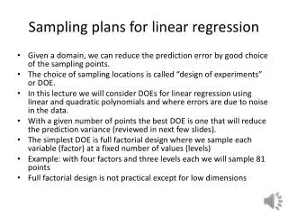
Sampling plans for linear regression • Given a domain, we can reduce the prediction error by good choice of the sampling points. • The choice of sampling locations is called “design of experiments” or DOE. • With a given number of points the best DOE is one that will reduce the prediction variance (reviewed in next few slides). • The simplest DOE is full factorial design where we sample each variable (factor) at a fixed number of values (levels) • Example: with four factors and three levels each we will sample 81 points • Full factorial design is not practical except for low dimensions
Linear Regression • Surrogate is linear combination of given shape functions • For linear approximation • Difference (error) between data and surrogate • Minimize square error • Differentiate to obtain
Model based error for linear regression • The common assumptions for linear regression • The true function is described by the functional form of the surrogate. • The data is contaminated with normally distributed error with the same standard deviation at every point. • The errors at different points are not correlated. • Under these assumptions, the noise standard deviation (called standard error) is estimated as • is used as estimate of the prediction error.
Prediction variance • Linear regression model • Define then • With some algebra • Standard error
Prediction variance for full factorial design • Recall that standard error (square root of prediction variance is • For full factorial design the domain is normally a box. • Cheapest full factorial design: two levels (not good for quadratic polynomials). • For a linear polynomial standard error is then • Maximum error at vertices • What does the ratio in the square root represent?
Quadratic Polynomials • A quadratic polynomial has (n+1)(n+2)/2 coefficients, so we need at least that many points. • Need at least three different values of each variable. • Simplest DOE is three-level, full factorial design • Impractical for n>5 • Also unreasonable ratio between number of points and number of coefficients • For example, for n=8 we get 6561 samples for 45 coefficients. • My rule of thumb is that you want twice as many points as coefficients
Central Composite Design • Includes 2n vertices, 2n face points plus ncrepetitions of central point • Can choose α so to • achieve spherical design • achieve rotatibility (prediction variance is spherical) • Stay in box (face centered) FCCCD • Still impractical for n>8
Repeated observations at origin • Unlike linear polynomials, prediction variance is high at origin. • Repetition at origin decreases variance there and improves stability (uniformity). • Repetition also gives an independent measure of magnitude of noise. • Can be used also for lack-of-fit tests.
Without repetition (9 points) • Contours of prediction variance for spherical CCD design.
Center repeated 5 times (13 points) . • With five repetitions we reduce the maximum prediction variance and greatly improve the uniformity. • Five points is the optimum for uniformity.
D-optimal design • Maximizes the determinant of XTX to reduce the volume of uncertainties about the coefficients. • Example: Given the model y=b1x1+b2x2, and the two data points (0,0) and (1,0), find the optimum third data point (p,q) in the unit square. • We have • So that the third point is (p,1), for any value of p • Finding D-optimal design in higher dimensions is a difficult optimization problem often solved heuristically
Matlab example >> ny=6;nbeta=6; >> [dce,x]=cordexch(2,ny,'quadratic'); >> dce' 1 1 -1 -1 0 1 -1 1 1 -1 -1 0 scatter(dce(:,1),dce(:,2),200,'filled') >> det(x'*x)/ny^nbeta ans = 0.0055 With 12 points: >> ny=12; >> [dce,x]=cordexch(2,ny,'quadratic'); >> dce' -1 1 -1 0 1 0 1 -1 1 0 -1 1 1 -1 -1 -1 1 1 -1 -1 0 0 0 1 scatter(dce(:,1),dce(:,2),200,'filled') >> det(x'*x)/ny^nbeta ans =0.0102
Problems DOE for regression • What are the pros and cons of D-optimal designs compared to central composite designs? • For a square, use Matlab to find and plot the D-optimal designs with 10, 15, and 20 points.
Space-Filling DOEs • Design of experiments (DOE) for noisy data tend to place points on the boundary of the domain. • When the error in the surrogate is due to unknown functional form, space filling designs are more popular. • These designs use values of variables inside range instead of at boundaries • Latin hypercubes uses as many levels as points • Space-filling term is appropriate only for low dimensional spaces. • For 10 dimensional space, need 1024 points to have one per orthant.
Monte Carlo sampling • Regular, grid-like DOE runs the risk of deceptively accurate fit, so randomness appeals. • Given a region in design space, we can assign a uniform distribution to the region and sample points to generate DOE. • It is likely, though, that some regions will be poorly sampled • In 5-dimensional space, with 32 sample points, what is the chance that all orthants will be occupied? • (31/32)(30/32)…(1/32)=1.8e-13.
Example of MC sampling • With 20 points there is evidence of both clamping and holes • The histogram of x1 (left) and x2 (above) are not that good either.
Latin Hypercube sampling • Each variable range divided into ny equal probability intervals. One point at each interval.
Latin Hypercube definition matrix • For n points with m variables: m by n matrix, with each column a permutation of 1,…,n • Examples • Points are better distributed for each variable, but can still have holes in m-dimensional space.
Improved LHS • Since some LHS designs are better than others, it is possible to try many permutations. What criterion to use for choice? • One popular criterion is minimum distance between points (maximize). Another is correlation between variables (minimize). • Matlablhsdesign uses by default 5 iterations to look for “best” design. • The blue circles were obtained with the minimum distance criterion. Correlation coefficient is -0.7. • The red crosses were obtained with correlation criterion, the coefficient is -0.055.
More iterations • With 5,000 iterations the two sets of designs improve. • The blue circles, maximizing minimum distance, still have a correlation coefficient of 0.236 compared to 0.042 for the red crosses. • With more iterations, maximizing the minimum distance also reduces the size of the holes better. • Note the large holes for the crosses around (0.45,0.75) and around the two left corners.
Reducing randomness further • We can reduce randomness further by putting the point at the center of the box. • Typical results are shown in the figure. • With 10 points, all will be at 0.05, 0.15, 0.25, and so on.
Problems LHS designs • Using 20 points in a square, generate a maximum-minimum distance LHS design, and compares its appearance to a D-optimal design. • Compare their maximum minimum distance and their det(XTX)