Download
1 / 24
390 likes | 1.83k Views
Time-of-Flight Mass Analyzers. Jonathan Karty C613 lecture 21 March 26, 2008. (Section 4.2 in Gross, pages 115-128). TOF Overview. Time-of-flight (TOF) is the least complex mass analyzer in terms of its theory

E N D
Time-of-Flight Mass Analyzers Jonathan Karty C613 lecture 21 March 26, 2008 (Section 4.2 in Gross, pages 115-128)
TOF Overview • Time-of-flight (TOF) is the least complex mass analyzer in terms of its theory • Ions are given a defined kinetic energy and allowed to drift through a field-free region (0.5 to several meters) • The time ions arrive at the detector is measured and related to the m/z ratio
TOF Concept • A packet of stationary ions is accelerated to a defined kinetic energy and the time required to move through a fixed distance is measured • First TOF design published in 1946 by W.E. Stephens Detector
TOF advantages • Theoretically unlimited mass range • Ions are not trapped (quad, IT, FTICR) nor are their flight paths curved (BE sectors) • Detection efficiencies induce practical limits of a few hundred kDa (M+H)+ • Instrument is not scanning (it is dispersive) • Analysis is very rapid (40+ kHz acquisition possible) • Wide range of m/z’s can be measured with good sensitivity • Moderate to high resolving powers (5,000-20,000+) • Moderate cost ($100k to $500k) • Relatively high duty cycle • Couples extremely well with pulsed ion sources (e.g. MALDI)
TOF Disadvantages • Requires high vacuum (<10-6 torr) • Coupling to continuous ion sources (e.g. ESI or EI) not straight forward • Requires complex and high speed electronics • High acceleration voltages (5-30 kV) • Fast detectors (ns or faster) • GHz sampling digital conversion • Large volumes of data can be generated quickly • Limited dynamic range • Often 102 or 103 at most • High resolution instruments can get rather large
Time-of-Flight Theory • From Physics 1: (1) KE = ½mv2 • From Physics 2: (2) KE = z*U = ½mv2 • All ions accelerated by the same voltage, U • From Physics 1: (3) ΔX= v0TOF + ½aTOF2 • (5) TOF = ΔX/v0 • 1,000 Th ion @ 19 kV, v ≈ 60 km/sec • ΔX same for all ions = D (flight tube length) • No acceleration in flight tube • TOF α U-1α (m/z)½
Mass Scale Calibration • TOF α (m/z)1/2 or m/z α TOF2 • Mass scale is calibrated measuring flight times known m/z ions and fitting them to a polynomial equation • (7) TOF = a*(m/z)1/2 + b also • Higher order calibrations are often used • 5th order on some commercial instruments • Form can be (7a) m/z = A*TOF2 + B*TOF + C
Resolution in TOF MS Easy way to improve resolution is to increase flight tube length (assuming excellent vacuum)
Real-world TOF MS • Previous examples all assumed ions formed at rest, at the same time, and all at the same position in the source • In reality, ions are formed throughout the source at various times, in various locations, with a range of initial kinetic energies • Practical TOF instrument design relies on minimizing the contributions of each of these realities
Influence of Initial Position • In EI, CI, and ESI sources, ions are NOT formed all in the exact same position • These differences in initial position have profound effects on the mass spectrum • Ions spend some time in the source prior to crusing through the flight tube • (14) TOFobs = TOFsource + TOFflight_tube • A more complete treatment of the TOF requires that we consider how the ions get accelerated
A brief discussion of acceleration • Ions are usually accelerated by using parallel plates at different potentials to create electric fields • Ions in an electric field gain energy according to the equation: (15) KE = z*(E*s) or U = z*(E*s) • z is charge, E is electric field strength in V/m, and s is distance the ion travels in the field (Lorentz force equation) • Time of flight in the source must be computed with a differential equation
0 V +100 V Initial Position Math
Starting Position Example • Both ions are 100 m/z (1.0364*10-6 kg/C) • Red ion is 6 mm from 0 V plate, blue ion is 5 mm from 0 V plate • s for red is 0.006 m; s for blue is 0.005 m • Distance between plates is 1 cm • Electric field is 10,000 V/m • Detector is 1 m from 2nd grid • TOFred = 94 usec TOFblue = 112 usec • Ered = 60 eV, Eblue = 50 eV Detector 0 V This effect tends to cause peaks to tail to longer TOF +100 V
Initial Kinetic Energy Spread • If the ion has a non-zero kinetic energy along the axis of the flight tube prior to acceleration: (25) KEtotal = z*U+U0(U0 is initial KE) • At 500 K, kT = 0.043 eV • Kinetic energies perpendicular to this axis can cause the ions to miss the detector entirely • The initial kinetic energy spread and initial position can be accounted for mathematically
How long do ions spend in the source? (initial KE and position) (initial direction) (uncertainty of ion formation)
Putting this all together • Source design is used to minimize the variables that contribute to peak broadening • High U to minimize U0 • Narrow ion formation regions to minimize s • Pulsing ions out of source to minimize t0
TOF designs to maximize resolving power • High acceleration voltages can reduce impact of initial KE distribution • Initial position effects are harder to minimize • Additional ion optical elements can be introduced to compensate for these two effects • Set flight tube axis perpendicular to major vector of KE distribution • orthogonal extraction
Time-lag focusing • There is a point in the flight tube where 2 ions starting at different positions arrive simultaneously • Adding a third grid allows the analyst to move this “focus plane” to the detector • 1955, Wiley and McLaren • 1994, Colby, King, and Reilly @ IU (special case for MALDI) • s0 is related to initial KE since all ions formed simultaneously +100 V +90 V Detector 0 V +100 V
Reflectrons? • In 1966, B. Mamyrin patented an ion mirror device for energy focusing and resolution improvement • A reflectron is a long series of electrodes that create an electric field to reverse the direction the ions travel • Higher energy ions spend more time in reflectron than lower energy ions • By adjusting parameters, ions with same m/z but slightly different KE’s can be made to arrive at a detector simultaneously
Reflectron drawing 0 V +110 V 0 V +100 V Detector
Reflectron Pros and Cons • Advantages • Focuses kinetic energies • Better resolution • Allows one to use same flight tube twice • Remember, res power increases with D • Cons • Only a narrow range of KE can be focused • Usually 85%-105% of E • Metastable ions are not focused by reflectron • If ion fragments in flight tube, products have same velocity as precursors (but KE is proportional to mass of product) • Reflectron focuses by energy
Measuring TOF Signals • Oscilloscope (aka multi-channel scaler) • Analog recorder (ion current vs. time) • Great for intense signals • Generates large data files (all times recorded) • Noise recorded as well as signal • Time to Digital Converter • Records only when an event occurred • Threshold is set so an event is arrival of 1 ion • Excellent for low signals (single ion counting) • Does NOT take into account intensity • 2 ions arriving simultaneously counts as 1 event • Limited dynamic range
Factors that Influence Resolution • Laser pulse width in MALDI • Detector response profile • Digitization rate and amplifier bandwidths • Kinetic energy distribution of ions • Initial position of ions in source • Power supply stability • Response profiles of pulsing electronics
Waters LCT Drawing Mass range: 60-20,000 m/z Resolving power: ~5,000 254 psec resolution TDC ESI or APCI source MS recorded at ~20 kHz Table-top MS (1.5x1x1 m) Cost ~$200,000