Download
1 / 37
370 likes | 492 Views
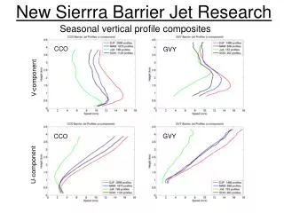
New Sierrra Barrier Jet Research. CCO. GVY. V-component. CCO. GVY. U-component. Seasonal vertical profile composites. American River Basin. Sheridan (60 m; SCPP).

E N D
New Sierrra Barrier Jet Research CCO GVY V-component CCO GVY U-component Seasonal vertical profile composites
American River Basin Sheridan (60 m; SCPP) Topography of California’s interior, including near the wind profilers at CCO & GVY and the American River Basin (which was also the taget area for SCPP (Parish 1982).
Three cross sections of the barrier-parallel isotachs (m s-1) measured within representative barrier jets over the American River Basin by the Wyoming King Air research aircraft (flight tracks depicted as dashed lines) and ground-based rawinsondes (including from Sheridan at x = 0, the site where serial ascents were released over seven winters) on 13 and 20 February 1979 (Parish 1982).
Time-height section of hourly wind profiles (flags = 25 m s-1; barbs = 5 m s-1; half-barbs = 2.5 m s-1) and color-coded signal-to-noise ratio measured by the Chico, California 915-MHz wind profiler during a representative barrier-jet event on 26 February 2004 (top panel). Companion time-series traces of surface wind speed (m s-1), pressure (mb), and rainfall (inches) are also shown (bottom panel).
(MWR 2005) (JHM 2007) (MWR 2008) Some recent relevant numerical model-centric articles that attempt to partially address the modulation of precipitation distributions by Sierra barrier jets.
Extensions of Smutz From Paul’s notes…. • Smutz had 3-hr resolution soundings in storms, we have 1-hr resolution wind profiles 24/7 for ~5-7 years. • Smutz had 300-m vertical sounding resolution; we have 100-m vertical resolution in our wind profiles. • Smutz does not show vertical structure composites of BJs… we will. • Smutz does not do a statistical analysis of BJ cases… just profiles. In contrast, with our hourly resolution profiler data, we do statistical analysis of both BJ profiles and BJ cases. With our cases we can asses mean BJ evolution. • Given 1-h resolution of wind profiles, we have many more observations of BJs (Smutz had 3-h soundings launched only during storms, whereas our hourly profiles were collected 24/7.) Hence, we can stratify our results much more effectively. • Given that we operated the wind profilers year-round, we can look at interseasonal variations in the occurrence and characteristics of the BJ. • Unlike Smutz, we have a dynamically consistent mesoscale dataset in the North American Regional Reanalysis (NARR) to do dynamical and precipitation composites. We can assess the BJ-precipitation relationship using NARR data. • We have hourly information on melting level behavior. • We have 2 different sites to look at spatial variability of barrier jets… one in the foothills and another at the base of the Sierra. Smutz only had the latter. • Our barrier jet constraints are more rigorous than Smutz’s barrier jet constraints.
Extension of Smutz Barrier Jet Climatology • Time resolution: • Smutz had 3-hrly soundings during wintertime storms; we have 1-hrly wind profiles 24/7 for 5-7 years. • Spatial variability: • Smutz analyzed data from one site at the base of the Sierra (Sheridan, CA); we have two sites: one at the base of the Sierra (Chico, CA) and another in the Sierra foothills (Grass Valley, CA). • Sample size: • Smutz had 1849 sounding profiles; we have 100,000+ wind profiles from two sites. • Our larger sample size allows us to stratify our results much more effectively. • Vertical resolution: • Smutz had 300-m vertical sounding resolution; we have 100-m vertical wind profile resolution. • Vertical structure: • Smutz did not analyze vertical structure composites… we will. • Statistical analysis: • Smutz does not do a statistical analysis of BJ cases… just profiles. • With our 1-hr wind profiles, we can do statistical analyses of both BJ profiles and BJ cases. • Through analysis of BJ cases, we can asses mean BJ evolution. • North American Regional Reanalysis data: • Unlike Smutz, we have a dynamically consistent mesoscale dataset in the NARR that can be used for dynamical and precipitation compositing. • We can assess the BJ-precipitation relationship using NARR data. • Melting layer: • We have hourly information on melting level. • Seasonal variation: • Since we operated the wind profilers year-round, we can look at interseasonal variations in the occurrence and characteristics of BJs. • BJ constraints: Our BJ constraints are more rigorous than Smutz’s BJ constraints.
Smutz Barrier Jet ConstraintsSheridan, CA (~60 m, msl) Before any analysis occurred, the coordinate axes were rotated 20° counter-clockwise from the cardinal directions such that 340° degrees becomes 0°. Barrier Jet Constraints: • Between 0.06 and 3.0 km • Relative v-component maximum (Vmax) is positive
Smutz Vmax height distribution Sheridan, CA (60 m, msl) # BJ Profiles = 1642 Mean = 1.12 km Median = 0.91 km Smutz 1986
Smutz Vmax distribution Sheridan, CA (60 m, msl) # BJ Profiles = 1642 Mean = 11.0 m/s Median = 9.4 m/s Smutz 1986
Wind Profiler Barrier Jet Profiler Constraints Before any analysis occurred, the coordinate axes were rotated 20° counter-clockwise from the cardinal directions such that 340° degrees becomes 0°. Barrier Jet Constraints: • Below 3 km • Maximum v-component (Vmax) wind speed > 12 m/s • Vmax wind direction between 70° and 250° • Above Vmax: (Vmax – v-component) > 2 m/s • Between Vmax and some v-component above Vmax there must be a decrease greater than 2 m/s • Below Vmax: (Vmax – v-component) > 0 m/s • Between Vmax and some v-component below Vmax there must be a decrease greater than 0 m/s • Vmax+1 > 0 m/s and Vmax-1 > 0 m/s • There must be data or interpolated data in the bins directly above and below Vmax • Vmax cannot occur in the 1st or last bin (between ground and 3 km) of the wind profiler data Note: For the case inventory, the above criteria had to persist for > 8 hours.
Vmax height distribution Chico, CA (41 m, msl) Sheridan, CA (Smutz 1986) Sheridan, CA (60 m, msl) # BJ Profiles = 1642 Mean = 1.12 km Median = 0.91 km # BJ Profiles = 6695 Mean = 1.11 km Median = 0.85 km Smutz 1986
Vmax distribution Sheridan, CA (60 m, msl) Chico, CA (41 m, msl) # BJ Profiles = 1642 Mean = 11.0 m/s Median = 9.4 m/s # BJ Profiles = 6695 Mean = 17.9 m/s Median = 15.9 m/s Smutz 1986
Vmax height distribution Chico, CA (41 m, msl) Grass Valley, CA (689 m, msl) Chico, CA (40 m, msl) # BJ profiles = 2563 Mean = 1.82 km Median = 1.80 km # BJ Profiles = 6695 Mean = 1.11 km Median = 0.85 km
Vmax distribution Chico, CA (41 m, msl) Grass Valley, CA (689 m, msl) # BJ Profiles = 6695 Mean = 17.9 m/s Median = 15.9 m/s # BJ profiles = 2563 Mean = 17.4 m/s Median = 15.8 m/s
Wind direction distribution at Vmax altitude Chico, CA (41 m, msl) Grass Valley, CA (689 m, msl) # BJ Profiles = 6695 Mean = 161.7° Median = 161.0° # BJ profiles = 2563 Mean = 173.7° Median = 174.0°
Wind speed distribution at Vmax altitude Chico, CA (41 m, msl) Grass Valley, CA (689 m, msl) # BJ Profiles = 6695 Mean = 18.44 m/s Median = 16.40 m/s # BJ profiles = 2563 Mean = 18.37 m/s Median = 17.00 m/s
U-component distribution at Vmax altitude Chico, CA (41 m, msl) Grass Valley, CA (689 m, msl) # BJ Profiles = 6695 Mean = 3.26 m/s Median = 2.72 m/s # BJ profiles = 2563 Mean = 4.84 m/s Median = 4.17 m/s
Monthly distribution Chico, CA (41 m, msl) Grass Valley, CA (689 m, msl) # BJ profiles = 6695 # BJ profiles = 2563
Barrier Jet Profiles Over ~7 years, 11.1% of the collected profiles at CCO satisfied the barrier jet constraints. Over ~5 years, 6.2% of the collected profiles at GVY satisfied the barrier jet constraints. 52.3% of the BJ profiles at CCO were accepted as BJ cases. 47.7% of the BJ profiles at GVY were accepted as BJ cases.
Distribution of range gate counts Chico, CA (41 m, msl) Grass Valley, CA (689 m, msl)
Seasonal vertical profile composites CCO GVY V-component CCO GVY U-component
Seasonal vertical profile composites GVY CCO Wind direction GVY CCO Wind speed
Barrier Jet Case Example #1 (CCO) transition
Barrier Jet Case Example #2 (CCO) transition
Double brightband in moments data during jump in melting-level altitude
NARR: Barrier Jet Case Example #1 – Before & after transition 12Z 12/15/02 – 09Z 12/16/02 15Z 12/16/02 – 06Z 12/17/02 500 mb Z (m) 925 mb Z (m)
NARR: Barrier Jet Case Example #1 – Before & after transition 12Z 12/15/02 – 09Z 12/16/02 15Z 12/16/02 – 06Z 12/17/02 IWV (mm) Accum. Precip. (mm)
NARR: Barrier Jet Case Example #1 – Before & after transition 12Z 12/15/02 – 09Z 12/16/02 15Z 12/16/02 – 06Z 12/17/02 925 mb V (m/s) 925 mb U (m/s)
NARR: Barrier Jet Case Example #1 – Before & after transition 12Z 12/15/02 – 09Z 12/16/02 15Z 12/16/02 – 06Z 12/17/02 925 mb T (deg C) 925 mb q (g/kg)
NARR: Barrier Jet Case Example #1 – Before & after transition 12Z 12/15/02 – 09Z 12/16/02 15Z 12/16/02 – 06Z 12/17/02 925 mb w (ub/s) 700 mb w (ub/s)
NARR: Barrier Jet Case Example #2 – Before & after transition 06Z 12/27/05 – 12Z 12/27/05 15Z 12/27/05 – 09Z 12/28/05 500 mb Z (m) 925 mb Z (m)
NARR: Barrier Jet Case Example #2 – Before & after transition 06Z 12/27/05 – 12Z 12/27/05 15Z 12/27/05 – 09Z 12/28/05 IWV (mm) Accum. Precip. (mm)
NARR: Barrier Jet Case Example #2 – Before & after transition 06Z 12/27/05 – 12Z 12/27/05 15Z 12/27/05 – 09Z 12/28/05 925 mb V (m/s) 925 mb U (m/s)
NARR: Barrier Jet Case Example #2 – Before & after transition 06Z 12/27/05 – 12Z 12/27/05 15Z 12/27/05 – 09Z 12/28/05 925 mb T (deg C) 925 mb q (g/kg)
NARR: Barrier Jet Case Example #2 – Before & after transition 06Z 12/27/05 – 12Z 12/27/05 15Z 12/27/05 – 09Z 12/28/05 925 mb w (ub/s) 700 mb w (ub/s)