Chapter 8 Multivariate Regression Analysis
Chapter 8 Multivariate Regression Analysis. 8.3 Multiple Regression with K Independent Variables 8.4 Significance tests of Parameters. Population Regression Model.

Chapter 8 Multivariate Regression Analysis
E N D
Presentation Transcript
Chapter 8Multivariate Regression Analysis 8.3 Multiple Regression with K Independent Variables 8.4 Significance tests of Parameters
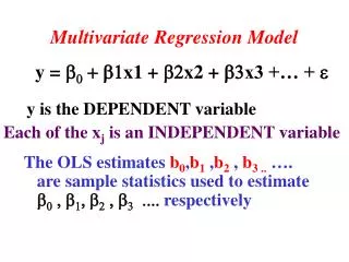
Population Regression Model The principles of bivariate regression can be generalized to a situation of several independent variables (predictors) of the dependent variable For K independent variables, the population regression and prediction models are: The sample prediction equation is:
Predict number of children ever born (Y) to the 2008 GSS respondents (N=1,906) as a linear function of education (X1), occup’l prestige (X2), no. of siblings (X3), and age (X4): People with more education and higher-prestige jobs have fewer children, but older people and those raised in families with many siblings have more children. Use the equation to predict the expected number of kids by a person with X1 = 12; X2 = 40; X3 = 8; X4 = 55: 2.04 For X1 = 16; X2 = 70; X3 = 1; X4 = 25: 0.71
OLS Estimation of Coefficients As with bivariate regression, the computer uses Ordinary Least Squares methods to estimate the intercept (a), slopes (bYX), and multiple coefficient of determination (R2) from sample data. OLS estimators minimize the sum of squared errors for the linear prediction: min See SSDA#4 Boxes 8.2 and 8.3 for details of best linear unbiased estimator (BLUE) characteristics and the derivations of OLS estimators for the intercept a and slope b
Nested Equations A set of nested regression equations successively adds more predictors to an equation to observe changes in their slopes with the dependent variable Predicting children ever born (Y) by adding education (X1); occupational prestige (X2); siblings (X3); age (X4). (Standard errors in parentheses) (1) (2) (3) (4)
F-test for 2 The hypothesis pair for the multiple coefficient of determination remains the same as in the bivariate case: But the F-test must also adjust the sample estimate of R2 for the df associated with the K predictors: As you enter more predictors into the equation in an effort to pump up your R2, you must pay the higher “cost” of an additional df per predictor to get that result.
Source dfR, dfE SS c.v. df MS F Regression 354.7 3 .05 3, 2.60 Error 5,011.1 1,910 .01 3, 3.78 Total 5,365.8 1,913 --------------------- .001 3, 5.42 Test the null hypothesis H0: 2 = 0 for Equation 3: 118.2 45.1 2.6 Decision about H0: _______________ RejectH0 Prob. Type I error: _______________ p < .001 Predictors account for more than 0% of children variance. Conclusion: ______________________________________
Difference in 2 for Nested Equations We can also test whether adding predictors to a second, nested regression equation increases 2: where subscripts “1” and “2” refer to the equations with fewer and more predictors, respectively The F-statistic tests whether adding predictors increases the population rho-square, relative to the difference in the two nested equations’ degrees of freedom:
dfR, dfE c.v. .05 1, 3.84 .01 1, 6.63 .001 1, 10.83 Is the 2 for Eq. 2 larger than the 2 forEq. 1? 2.0 Don’t Reject H0 Decision:_________________ Prob. Type I error: __________ Interpretation:Adding occupation to the regression equation with education did not significantly increase the explained variance in number of children ever born. In the population, the two coefficients of determination are equal; each explains about 5% of the variance of Y.
dfR, dfE c.v. .05 1, 3.84 .01 1, 6.63 .001 1, 10.83 Now test the difference in 2 for Eq. 4 versus Eq. 3: 299.2 Reject H0 Decision:_________________ p < .001 Prob. Type I error: __________ Interpretation:Adding age to the regression equation with three other predictors greatly increases the explained variance in number of children ever born. The coefficient of determination for equation #4 seems to be almost three times larger than for equation #3.
Adjusting R2 for K predictors The meaning of the multiple regression coefficient of determination is identical to the bivariate case: However, when you report the sample estimate of a multiple regression R2, you must adjust its value by 1 degree of freedom for each of the K predictors: For large sample N and low R2, not much will change.
Eq. R2 K Adj. R2 1: 0.051 1 2: 0.052 2 3: 0.066 3 4: 0.193 4 Adjust the sample R2 for each of the four nested equations (N = 1,906): 0.0505 0.0510 0.0645 0.1913
Here are those four nested regression equations again with the number of ever-born children as the dependent variable. Now we’ll examine their regression slopes. Predict children ever born (Y) by adding education (X1); occupational prestige (X2); siblings (X3); age (X4) (Standard errors in parentheses) (1) (2) (3) (4)
Interpreting Nested byx • The multiple regression slopes are partial or net effects. When other independent variables are statistically “held constant,” the size of bYX often decreases. These changes occur if predictor variables are correlated with each other as well as with the dependent variable. • Two correlated predictors divide their joint impact on the dependent variable between both byxcoefficients. For example, age and education are negatively correlated (r = -.17): older people have less schooling. When age was entered into equation #4, the net effect of education on number of children decreased from b1 = -.124 to b1 = -.080. So, controlling for respondent’s age, an additional year of education decreases the number of children ever born by a much smaller amount.
t-test for Hypotheses about t-test for hypotheses about K predictors uses familiar procedures A hypothesis pair about the population regression coefficient for jth predictor could haveatwo-tailed hypothesis: Or, a hypothesis pair could indicate the researcher’s expected direction (sign) of the regression slope: Testing an hypothesis about j uses a t-test with N-K-1 degrees of freedom (i.e., a Z-test for a large sample) where bj is the sample regression coefficient & denominator is the standard error of the sampling distribution of j (see formula in SSDA#4, p. 266)
1-tail 2-tail .05 1.65 1.96 .01 2.33 2.58 .001 3.10 3.30 Here are two hypotheses, about education (1) and occupational prestige (2), to be tested using Eq, 4: Test a two-tail hypothesis about 1: -5.71 Reject H0 p < .001 Decision: ______________ Prob. Type I error: ________ Test a one-tail hypothesis about 2: -0.33 Don’t reject H0 Decision: ______________ Prob. Type I error: ________
Test one-tailed hypotheses about expected positive effects siblings (3) and age (4) on number of children ever born: +6.09 Reject H0 p < .001 Decision: ______________ Prob. Type I error: ________ +17.50 Reject H0 p < .001 Decision: ______________ Prob. Type I error: ________ Interpretation:These sample regression statistics are very unlikely to come from a population whose regression parameters are zero (j= 0).
Standardizing regression slopes (*) Comparing effects of predictors on a dependent variable is difficult, due to differences in units of measurement Beta coefficient (*) indicates effect of an X predictor on the Y dependent variable in standard deviation units • Multiply the bYX for each Xi by that predictor’s standard deviation • Divide by the standard deviation of the dependent variable, Y The result is a standardized regression equation, written with Z-score predictors, but no intercept term:
Standardize the regression coefficients in Eq. 4 Variable s.d. Y Children 1.70 X1 Educ. 3.08 X2 Occup. 13.89 X3 Sibs 3.19 X4 Age 17.35 Use these stnd. devs. to change all the bYX to *: -0.14 -0.01 +0.13 +0.36 Write the standardized equation:
Interpreting * Standardizing regression slopes transforms predictors’ effects on the dependent variable from their original measurement units into standard-deviation units. Hence, you must interpret and compare the * effects in standardized terms: Education * = -0.14 a 1-standard deviation difference in education levels reduces the number of children born byone-seventhst. dev. Occupational * = -0.01 a 1-standard deviation difference in prestige reduces N of children born byone-hundredthst. dev. Siblings * = +0.13 a 1-standard deviation difference in siblings increases the number of children born byone-eighthst. dev. Age * = +0.36 a 1-standard deviation difference in age increases the number of children born by more thanone-thirdst. dev. Thus, age has the largest effect on number of children ever born; occupation has the smallest impact (and it’s not significant)
Let’s interpret a standardized regression, where annual church attendance is regressed on X1 = religious intensity (a 4-point scale), X2 = age, and X3 = education: The standardized regression equation: • Interpretations: • Only two predictors significantly increase church attendance • The linear relations explain 26.9% of attendance variance • Religious intensity has strongest effect (1/2 std. deviation) • Age effect on attendance is much smaller (1/12 std. dev.)
Dummy Variables in Regression Many important social variables are not continuous but measured as discrete categories and thus cannot be used as independent variables without recoding Examples of such variables include gender, race, religion, marital status, region, smoking, drug use, union membership, social class, college graduation Dummy variablecoded “1” to indicate the presence of an attribute and “0” its absence • Create & name one dummy variable for each of the K categories of the original discrete variable 2. For each dummy variable, code a respondent “1” if s/he has that attribute, “0” if lacking that attribute 3. Every respondent will have a “1” for only one dummy, and “0” for the K-1 other dummy variables
Recode SEX as two new dummies MARITAL MARRYD WIDOWD MALE DIVORCD FEMALE SEPARD NEVERD 1 = Men 1 0 1 = Married 1 0 0 0 0 2 = Widowed 0 1 0 0 0 2 = Women 0 1 3 = Divorced 0 0 1 0 0 4 = Separated 0 0 0 1 0 5 = Never 0 0 0 0 1 GSS codes for SEX are arbitrary: 1 = Men & 2 = Women MARITAL five categories from 1 = Married to 5 = Never
RECODE MARRYD WIDOWD DIVORD SEPARD NEVERD 1 972 164 281 70 531 0 1,046 1,854 1,737 1,948 1,487 TOTAL 2,018 2,018 2,018 2,018 2,018 SPSS RECODE to create K dummy variables (1-0) from MARITAL The ORIGINAL 2008 GSS FREQUENCIES: RECODE STATEMENTS: COMPUTE marryd=0. COMPUTE widowd=0. COMPUTE divord=0. COMPUTE separd=0. COMPUTE neverd=0. IF (marital EQ 1) marryd=1. IF (marital EQ 2) widowd=1. IF (marital EQ 3) divord=1. IF (marital EQ 4) separd=1. IF (marital EQ 5) neverd=1. Every case is coded 1 on one dummy variable and 0 on the other four dummies. The MARITAL category frequencies above appear in the “1” row for the five marital status dummy variables below:
Linear Dependency among Dummies Given K dummy variables, if you know a respondent’s codes for K - 1 dummies, then you also know that person’s code for the Kth dummy! This linear dependency is similar to the degrees of freedom problem in ANOVA. Thus, to use a set of K dummy variables as predictors in a multiple regression equation, you must omit one of them. Only K-1 dummies can be used in an equation. The omitted dummy category serves as the reference category (or baseline), against which to interpret the K-1 dummy variable effects (b) on the dependent variable
Use four of the five marital status dummy variables to predict annual sex frequency in 2008 GSS.WIDOWD is the omitted dummy, serving as the reference category. Widowsare coded “0” on all four dummies, so their prediction is: 8.8 61.2 41.6 29.9 61.8 Married: Divorced: Separated: Never: Which persons are the least sexually activity? Which the most?
ANCOVA Analysis of Covariance (ANCOVA)equation has both dummy variable and continuous predictors of a dependent variable Marital status is highly correlated with age (widows are older, never marrieds are younger), and annual sex activity falls off steadily as people get older. Look what happens to the marital effects when age is controlled, by adding AGE to the marital status predictors of sex frequency: • Each year of age reduces sex by –1.7 times per year. • Among people of same age, marrieds have more sex than others, but never marrieds now have less sex than widows! • What would you predict for: Never marrieds aged 22? Marrieds aged 40? Widows aged 70?
Add FEMALE dummy to regression of church attendance on X1 = religious intensity, X2 = age, and X3 = education: The standardized regression equation: • Interpretations: • Women attend church 2.20 times more per year than men • Other predictors’ effects unchanged when gender is added • Age effect is twice as larger as gender effect • Religious intensity remains strongest predictor of attendance