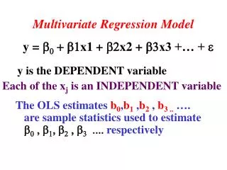
Multivariate Regression Analysis
Multivariate Regression Analysis. Aim. Establish a predictive model between one or more response variables and one or more input variables. Measurement. Response. Areas where Regression Analysis is useful. Process and Environmental Monitoring Process Control


Multivariate Regression Analysis
E N D
Presentation Transcript
Aim • Establish a predictive model between one or more response variables and one or more input variables Measurement Response
Areas where Regression Analysis is useful • Process and Environmental Monitoring • Process Control • Product Quality/Product Properties
Why? • Reveal correspondences/correlations • Increased Accuracy/Precision in the Information Process • Improved (reduced) Response time in the Information Process (“on-line”, “at-line”)
How? 1. Collect Data 2. Analyse Data 3. Establish a Predictive Model Y = BX, yi = f (x1, x2, .., xm) y = bx, y = f (x1, x2, .., xm)
m y = X + e b m n n m ^ y = Xb Multivariate Regression Model: y = Xb + e
The solution of regression problems y = Xb + e When e is minimised: y = Xb Xty = XtXb The “Normal equation”:(XtX)-1Xty = b Minimise with respect to b0, b1,…,bM Condition: XtX must have full rank
Problems • Many x-variables, few objects (measurements) • Correlation between the x-variables det |XtX | 0 (XtX)-1 does not exist! • “Noise” in X
Generalised inverse Generalised inverse:X+ = (XtX)-1Xt Normal equation: b = X+y Biased Regression Methods differ in the way that the Generalised Inverse is calculated
Problem Specification Standards with known concentrations are measured on two highly correlated wavelength. Make a calibration model between the concentrations and the measured intensities at the two wavelengths: c = f(x1,x2)
x2 7 PC1 5 t1 6 t2 x1 3 . 4 . . 1 tN 2 Dimensionality Reduction t, score vector c, concentration vector Quantitative information about the concentration in t
PC1 y ^ ^ y1 t1 = bPC1 t2 y2 . . ^ . . t = f(x1, x2) = f(c) . . tN yN The Regression
^ ^ t1 y1 = bPC1 y - y = bPC1t + e t2 y2 . . ^ . . . . yN tN tt(y - y ) bPC1 = ttt Calculation of the Regression Coefficient
Response (output) variable System y Instrumental (spectral) variables I y = f(X) I X Regression modelling
A X = TPt + E = tapat + E a=1 A y = y+bata + e a=1 Solution 1. Decompose the matrix of spectral data (X) into (orthogonal) latent variables (LVs) 2. Model the dependent variable in terms of the latent-variable score vectors
Scores: t = f (c1, c2, …) Contains quantitative info about the concentrations Loadings: p= f (1, 2, …) Contains qualitative info about the spectra Scores and Loadings
Partial Least Squares (PLS) - best for prediction Principal Component Regression (PCR) - best for outlier checking Regression Methods Combine the methods
= bLV t1 t2 tA y-y orthogonal y = y + bLV1t1 + bLV1t2 + .. + bLVAtA Data described by several Latent Variables Model:
A y - y = bLV,ata + e a=1 A tbt(y - y)= bLV,a tbttLVa + e a=1 zero, except for a=b (y - y)tbt bLV,B= tbt tb Calculation of the regression vector
Latent-Variable Regression Modelling The Modelling process Validation Interpretation (Regr. coeff., loadings) Number oflatent variables (Explained var. in X and Y, Cross Validation, Regr. Coeff., Loadings etc.) OutlierDetection
Cross Validation (statistical validation) i) Divide the samples into a number of groups, ng. ii) For each LV dimension, a=1,2,.., A+1, perform the following calculations:1. Estimate the LV a with group k of samples excluded. 2. Predict the responses for samples in group k. 3. Calculate the squared prediction error for the left-out samples, iii) Repeat step ii)until all samples have been kept out once, and only once, then calculate iv) If SEP(a)<SEP(a-1) go to ii), otherwise stop and select number of dimensions (LVs) in model as a-1, A
Application Example 1 Process industry, where the principal qualities1 of products are linked to chemical composition of raw material and the manufacturing process. 1 O. M. Kvalheim, Chemom. & Intel. Lab. Syst. 19 (1993) iii-iv.
Application Example 2 Environmental sciences, such as the prediction of the diversity of a biological system from instrumental fingerprinting of the chemical environment, principal environmental responses.