Download
1 / 38
380 likes | 406 Views
Investigating loss of stability in heavily loaded transmission corridors and adapting bifurcation tools for interarea swing modes. Key ideas, questions, caveats, and computational formulations discussed.

E N D
Network Structure in Swing Mode Bifurcations • Motivation & Background • Practical Goal: examine loss of stability mechanisms associated w/ heavily loaded transmission corridors. • Expect presence of low frequency, interarea swing modes across transmission corridor. • Can bifurcation tools developed for voltage analysis be adapted to this scenario (are voltage & angle instabilities really that different)?
Key Ideas • Voltage methods typically assume one degree of freedom path in “parameter space” (e.g. load), or seek “closest” point in parameter space at which bifurcations occur • Alternative: leave larger # of degrees of freedom in parameter space, but constrain structure of eigenvector at bifurcation.
Key Questions • Is there a priori knowledge of form of eigenvector of interest for “mode” of instability we’re after? • Precisely what formulation for matrix who’s eigenvector/eigenvalue is constrained (e.g., what generator model, what load model, how is DAE structure treated, etc.)
Caveats (at present...) • Development to date uses only very simple, classical model for generators. • Previous work in voltage stability shows examples in which “earlier” loss of stability missed by such a simple model (e.g. Rajagopalan et al, Trans. on P.S. ‘92).
Review - Relation of PF Jacobian and Linearized Dynamic Model • This issue well treated in existing literature, but still useful to develop notation suited to generalized eigenvalue problem. • Structure in linearization easiest to see if we keep all phase angles as variables; neglect damping/governor; assume lossless transmission & symmetric PF Jac. Relax many of these assumptions in computations.
Review - Relation of PF Jacobian and Linearized Dynamic Model • Form of nonlinear DAE model
Review - Relation of PF Jacobian and Linearized Dynamic Model • Requisite variable/function definitions:
Review - Relation of PF Jacobian and Linearized Dynamic Model • variable/function definitions:
Review - Relation of PF Jacobian and Linearized Dynamic Model • variable/function definitions:
Linearized DAE/”Singular System” Form • Write linearization as:
Component Definitions • where:
Component Definitions é ù I • and: 0 0 m x m ê ú S J J = 0 1 1 1 2 ë û J J 0 2 1 2 2 n n-m (2n-m)x(2n-m) J J : x , = I R I R I R ® é ù N N ¶ P ¶ P ¶ V ê ¶ d ú L N N I ë û ¶ Q ¶ { Q - Q } ¶ V ¶ d L
Relation to Reduced Dimension Symmetric Problem • Consider reduced dimension, symmetric generalized eigenvalue problem defined by pair (E, J), where:
Relation to Reduced Dimension Symmetric Problem • FACT: Finite generalized eigenvalues of (E, J) completely determine finite generalized eigenvalues of
Relation to Reduced Dimension Symmetric Problem • In particular,
Key Observation • In seeking bifurcation in full linearized dynamics, we may work with reduced dimension, symmetric generalized eigenvalue problem whose structure is determined by PF Jacobian & inertias. • When computation (sparsity) not a concern, equivalent to e.v.’s of
Role of Network Structure • Question: what is a mechanism by which might drop rank? • First, observe that under lossless network approximation, the reduced Jacobian has admittance matrix structure; i.e. diagonal elements equal to – {sum of off-diagonal elements}.
Role of Network Structure • Given this admittance matrix structure, reduced PF Jacobianhas associated network graph. • A mechanism for loss of rank can then be identified: branches forming a cutset all have weights of zero.
Role of Network Structure • Eigenvector associated with new zero eigenvalue is identifiable by inspection:where is a positive real constant, and partition of eigenvector is across the cutset.
Role of Network Structure • Returning to associated generalized eigenvalue problem, to preserve sparsity, one would have:
Role of Network Structure • Finally, in original generalized eigenvalue problem for full dynamics, the new eigenvector has structure [ 1 , – 1 ] in components associated with generator phase angles. • Strongly suggests an inter area swing mode, with gens on one side of cutset 180º out of phase with those on other side.
Summary so far... • Exploiting on a number of simplifying assumptions (lossless network, symmetric PF Jacobian, classical gen model...), identify candidate structure for eigenvector associated with a “new” eigenvalue at zero. • Look for limiting operating conditions that yield J realizing this bifurcation & e-vector.
Computational Formulation • Very analogous to early “direct” methods of finding loading levels associated with Jacobian singularity in voltage collapse literature (e.g., Alvarado/Jung, 88). • But instead of leaving eigenvector components associated with zero eigenvalue as free variables, we constrain components associated with gen angles.
Computational Formulation • Must compensate with “extra” degrees of freedom. • For example to follow, generation dispatch selected as new variables. Clearly, many other possible choices...
Computational Formulation • Final observation: while it is convenient to keep all angles as variables in original analysis, in computation we select a reference angle and eliminate that variable. • Resulting structure of gen angle e-vector components becomes [ 0 , 1 ]
Computational Formulation • Simultaneous equations to be solved: • Note that f tilde terms are power balance equations, deleting gen buses. Once angles & voltages solved, gen dispatch is output.
Computational Formulation • Solution method is full Newton Raphson. • Aside: the Jacobian of these constraint equations involves 2nd order derivative of PF equations. Solutions routines developed offer very compact & efficient vector evaluations of higher order PF derivative.
Case Study • Based on modified form of IEEE 14 bus test system.
14 Bus Test System 13 - Transmission Line #'s # 19 20 - Bus #'s # 12 14 13 11 17 11 G 10 12 1 18 8 16 14 15 2 9 6 G G 9 10 7 8 4 7 1 5 5 6 2 4 3 3 G G Cutset Here
Case Study • N-R Initialization: initial operating point selected heuristically at present. Simply begin from op. pnt. that loads up a transmission corridor, with gens each side. • Here choice has gens 1, 2, 3 on one side, gens 6, 8 on other side. • Model has rotational damping added as rough approximation to governor action.
Future Work • Key question 1: must systems inevitably encounter loss of stability via flux decay/voltage control mode (as identified in Rajagopalan et al) before this type of bifurcation? • Hypothesis: perhaps not if good reactive support throughout system as transmission corridor is loaded up.
Future Work • Key question 2: possibility of same weakness as direct point of collapse calculations in voltage literature - many generators hitting reactive power limits along the loading path. • Answer will be closely related to that of question 1!
Conclusions • Simple exercise to shift focus back from bifurcations primarily associated w/ voltage, to bifurcations primarily associated with swing mode. • Key idea: hypothesize a form for eigenvector, restrict search for bifurcation point to display that eigenvector.
Conclusions • While further is clearly development needed, method here could provide simple computation to identify a stability constraint on ATC across a transmission corridor.