Download

1 / 60
600 likes | 625 Views
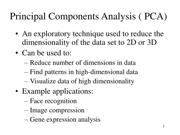
Learn about Principal Components Analysis (PCA), a technique to summarize variance-covariance structures of variables, visualize data, reduce dimensionality, and more. Explore examples and applications of PCA in data classification, noise reduction, trend analysis, and factor analysis procedures.

E N D
Principal Components Analysis on Images and Face Recognition Most Slides by S. Narasimhan
Example: 53 Blood and urine measurements (wet chemistry) from 65 people (33 alcoholics, 32 non-alcoholics). Matrix Format Spectral Format Data Presentation
Data Presentation Univariate Bivariate Trivariate
Data Presentation • Better presentation than ordinate axes? • Do we need a 53 dimension space to view data? • How to find the ‘best’ low dimension space that conveys maximum useful information? • One answer: Find “Principal Components”
All principal components (PCs) start at the origin of the ordinate axes. First PC is direction of maximum variance from origin Subsequent PCs are orthogonal to 1st PC and describe maximum residual variance Principal Components 30 25 20 Wavelength 2 PC 1 15 10 5 0 0 5 10 15 20 25 30 Wavelength 1 30 25 20 PC 2 Wavelength 2 15 10 5 0 0 5 10 15 20 25 30 Wavelength 1
The Goal We wish to explain/summarize the underlying variance-covariance structure of a large set of variables through a few linear combinations of these variables.
Uses: Data Visualization Data Reduction Data Classification Trend Analysis Factor Analysis Noise Reduction Examples: How many unique “sub-sets” are in the sample? How are they similar / different? What are the underlying factors that influence the samples? Which time / temporal trends are (anti)correlated? Which measurements are needed to differentiate? How to best present what is “interesting”? Which “sub-set” does this new sample rightfully belong? Applications
Trick: Rotate Coordinate Axes Suppose we have a population measured on p random variables X1,…,Xp. Note that these random variables represent the p-axes of the Cartesian coordinate system in which the population resides. Our goal is to develop a new set of p axes (linear combinations of the original p axes) in the directions of greatest variability: X2 X1 This is accomplished by rotating the axes.
Algebraic Interpretation • Given m points in a n dimensional space, for large n, how does one project on to a low dimensional space while preserving broad trends in the data and allowing it to be visualized?
Algebraic Interpretation – 1D • Given m points in a n dimensional space, for large n, how does one project on to a 1 dimensional space? • Choose a line that fits the data so the points are spread out well along the line
Algebraic Interpretation – 1D • Formally, minimize sum of squares of distances to the line. • Why sum of squares? Because it allows fast minimization, assuming the line passes through 0
Algebraic Interpretation – 1D • Minimizing sum of squares of distances to the line is the same as maximizing the sum of squares of the projections on that line, thanks to Pythagoras.
PCA: General From k original variables: x1,x2,...,xk: Produce k new variables: y1,y2,...,yk: y1 = a11x1 + a12x2 + ... + a1kxk y2 = a21x1 + a22x2 + ... + a2kxk ... yk = ak1x1 + ak2x2 + ... + akkxk such that: yk's are uncorrelated (orthogonal) y1 explains as much as possible of original variance in data set y2 explains as much as possible of remaining variance etc.
2nd Principal Component, y2 1st Principal Component, y1
xi2 yi,1 yi,2 xi1 PCA Scores
λ2 λ1 PCA Eigenvalues
PCA: Another Explanation From k original variables: x1,x2,...,xk: Produce k new variables: y1,y2,...,yk: y1 = a11x1 + a12x2 + ... + a1kxk y2 = a21x1 + a22x2 + ... + a2kxk ... yk = ak1x1 + ak2x2 + ... + akkxk yk's are Principal Components such that: yk's are uncorrelated (orthogonal) y1 explains as much as possible of original variance in data set y2 explains as much as possible of remaining variance etc.
Principal Components Analysis on: • Covariance Matrix: • Variables must be in same units • Emphasizes variables with most variance • Mean eigenvalue ≠ 1.0 • Correlation Matrix: • Variables are standardized (mean 0.0, SD 1.0) • Variables can be in different units • All variables have same impact on analysis • Mean eigenvalue = 1.0
PCA: General {a11,a12,...,a1k} is 1st Eigenvector of correlation /covariance matrix, and coefficients of first principal component {a21,a22,...,a2k} is 2nd Eigenvector of correlation/covariance matrix, and coefficients of 2nd principal component … {ak1,ak2,...,akk} is kth Eigenvector of correlation/covariance matrix, and coefficients of kth principal component
Dimensionality Reduction • Dimensionality reduction • We can represent the orange points with only their v1 coordinates • since v2 coordinates are all essentially 0 • This makes it much cheaper to store and compare points • A bigger deal for higher dimensional problems
PCA Example – STEP 1 • Subtract the mean from each of the data dimensions. All the x values have x subtracted and y values have y subtracted from them. This produces a data set whose mean is zero. Subtracting the mean makes variance and covariance calculation easier by simplifying their equations. The variance and co-variance values are not affected by the mean value.
PCA Example – STEP 1 http://kybele.psych.cornell.edu/~edelman/Psych-465-Spring-2003/PCA-tutorial.pdf
PCA Example – STEP 1 http://kybele.psych.cornell.edu/~edelman/Psych-465-Spring-2003/PCA-tutorial.pdf DATA: x y 2.5 2.4 0.5 0.7 2.2 2.9 1.9 2.2 3.1 3.0 2.3 2.7 2 1.6 1 1.1 1.5 1.6 1.1 0.9 ZERO MEAN DATA: x y .69 .49 -1.31 -1.21 .39 .99 .09 .29 1.29 1.09 .49 .79 .19 -.31 -.81 -.81 -.31 -.31 -.71 -1.01
PCA Example –STEP 2 • Calculate the covariance matrix cov = .616555556 .615444444 .615444444 .716555556 • since the non-diagonal elements in this covariance matrix are positive, we should expect that both the x and y variable increase together.
PCA Example –STEP 3 • Calculate the eigenvectors and eigenvalues of the covariance matrix eigenvalues = 0.049083399 1.28402771 eigenvectors = -.735178656 -.677873399 .677873399 -.735178656
PCA Example –STEP 3 http://kybele.psych.cornell.edu/~edelman/Psych-465-Spring-2003/PCA-tutorial.pdf • eigenvectors are plotted as diagonal dotted lines on the plot. • Note they are perpendicular to each other. • Note one of the eigenvectors goes through the middle of the points, like drawing a line of best fit. • The second eigenvector gives us the other, less important, pattern in the data, that all the points follow the main line, but are off to the side of the main line by some amount.
PCA Example –STEP 4 • Reduce dimensionality and form feature vector the eigenvector with the highest eigenvalue is the principle component of the data set. In our example, the eigenvector with the largest eigenvalue was the one that pointed down the middle of the data. Once eigenvectors are found from the covariance matrix, the next step is to order them by eigenvalue, highest to lowest. This gives you the components in order of significance.
PCA Example –STEP 4 Now, if you like, you can decide to ignore the components of lesser significance. You do lose some information, but if the eigenvalues are small, you don’t lose much • n dimensions in your data • calculate n eigenvectors and eigenvalues • choose only the first p eigenvectors • final data set has only p dimensions.
PCA Example –STEP 4 • Feature Vector FeatureVector = (eig1 eig2 eig3 … eign) We can either form a feature vector with both of the eigenvectors: -.677873399 -.735178656 -.735178656 .677873399 or, we can choose to leave out the smaller, less significant component and only have a single column: - .677873399 - .735178656
PCA Example –STEP 5 • Deriving the new data FinalData = RowFeatureVector x RowZeroMeanData RowFeatureVector is the matrix with the eigenvectors in the columns transposed so that the eigenvectors are now in the rows, with the most significant eigenvector at the top RowZeroMeanData is the mean-adjusted data transposed, ie. the data items are in each column, with each row holding a separate dimension.
PCA Example –STEP 5 FinalData transpose: dimensions along columns x y -.827970186 -.175115307 1.77758033 .142857227 -.992197494 .384374989 -.274210416 .130417207 -1.67580142 -.209498461 -.912949103 .175282444 .0991094375 -.349824698 1.14457216 .0464172582 .438046137 .0177646297 1.22382056 -.162675287
PCA Example –STEP 5 http://kybele.psych.cornell.edu/~edelman/Psych-465-Spring-2003/PCA-tutorial.pdf
Reconstruction of original Data • If we reduced the dimensionality, obviously, when reconstructing the data we would lose those dimensions we chose to discard. In our example let us assume that we considered only the x dimension…
Reconstruction of original Data http://kybele.psych.cornell.edu/~edelman/Psych-465-Spring-2003/PCA-tutorial.pdf x -.827970186 1.77758033 -.992197494 -.274210416 -1.67580142 -.912949103 .0991094375 1.14457216 .438046137 1.22382056
Appearance-based Recognition • Directly represent appearance (image brightness), not geometry. • Why? Avoids modeling geometry, complex interactions between geometry, lighting and reflectance. • Why not? Too many possible appearances! m “visual degrees of freedom” (eg., pose, lighting, etc) R discrete samples for each DOF How to discretely sample the DOFs? How to PREDICT/SYNTHESIS/MATCH with novel views?
Appearance-based Recognition • Example: • Visual DOFs: Object type P, Lighting Direction L, Pose R • Set of R * P * L possible images: • Image as a point in high dimensional space: is an image of N pixels and A point in N-dimensional space Pixel 2 gray value Pixel 1 gray value
= + The Space of Faces • An image is a point in a high dimensional space • An N x M image is a point in RNM • We can define vectors in this space as we did in the 2D case [Thanks to Chuck Dyer, Steve Seitz, Nishino]
Key Idea • Images in the possible set are highly correlated. • So, compress them to a low-dimensional subspace that • captures key appearance characteristics of the visual DOFs. • EIGENFACES: [Turk and Pentland] USE PCA!
Eigenfaces Eigenfaces look somewhat like generic faces.
Problem: Size of Covariance Matrix A • Suppose each data point is N-dimensional (N pixels) • The size of covariance matrix A is N x N • The number of eigenfaces is N • Example: For N = 256 x 256 pixels, Size of A will be 65536 x 65536 ! Number of eigenvectors will be 65536 ! Typically, only 20-30 eigenvectors suffice. So, this method is very inefficient!
Eigenfaces – summary in words • Eigenfaces are the eigenvectors of the covariance matrix of the probability distribution of the vector space of human faces • Eigenfaces are the ‘standardized face ingredients’ derived from the statistical analysis of many pictures of human faces • A human face may be considered to be a combination of these standardized faces
Generating Eigenfaces – in words • Large set of images of human faces is taken. • The images are normalized to line up the eyes, mouths and other features. • Any background pixels are painted to the same color. • The eigenvectors of the covariance matrix of the face image vectors are then extracted. • These eigenvectors are called eigenfaces.
Eigenfaces for Face Recognition • When properly weighted, eigenfaces can be summed together to create an approximate gray-scale rendering of a human face. • Remarkably few eigenvector terms are needed to give a fair likeness of most people's faces. • Hence eigenfaces provide a means of applying data compression to faces for identification purposes.
Dimensionality Reduction The set of faces is a “subspace” of the set of images • Suppose it is K dimensional • We can find the best subspace using PCA • This is like fitting a “hyper-plane” to the set of faces • spanned by vectors v1, v2, ..., vK Any face:
Eigenfaces • PCA extracts the eigenvectors of A • Gives a set of vectors v1, v2, v3, ... • Each one of these vectors is a direction in face space • what do these look like?
Projecting onto the Eigenfaces • The eigenfaces v1, ..., vK span the space of faces • A face is converted to eigenface coordinates by
Recognition with Eigenfaces • Algorithm • Process the image database (set of images with labels) • Run PCA—compute eigenfaces • Calculate the K coefficients for each image • Given a new image (to be recognized) x, calculate K coefficients • Detect if x is a face • If it is a face, who is it? • Find closest labeled face in database • nearest-neighbor in K-dimensional space
Key Property of Eigenspace Representation • Given • 2 images that are used to construct the Eigenspace • is the eigenspace projection of image • is the eigenspace projection of image • Then, • That is, distance in Eigenspace is approximately equal to the • correlation between two images.
i = K NM Choosing the Dimension K eigenvalues • How many eigenfaces to use? • Look at the decay of the eigenvalues • the eigenvalue tells you the amount of variance “in the direction” of that eigenface • ignore eigenfaces with low variance