Download
1 / 15
150 likes | 168 Views
This article explains how to use the Hilbert Transform to gain insights into the phase of propagation of a phenomenon. It also demonstrates the application of the Hilbert Transform on a time series signal using MATLAB.

E N D
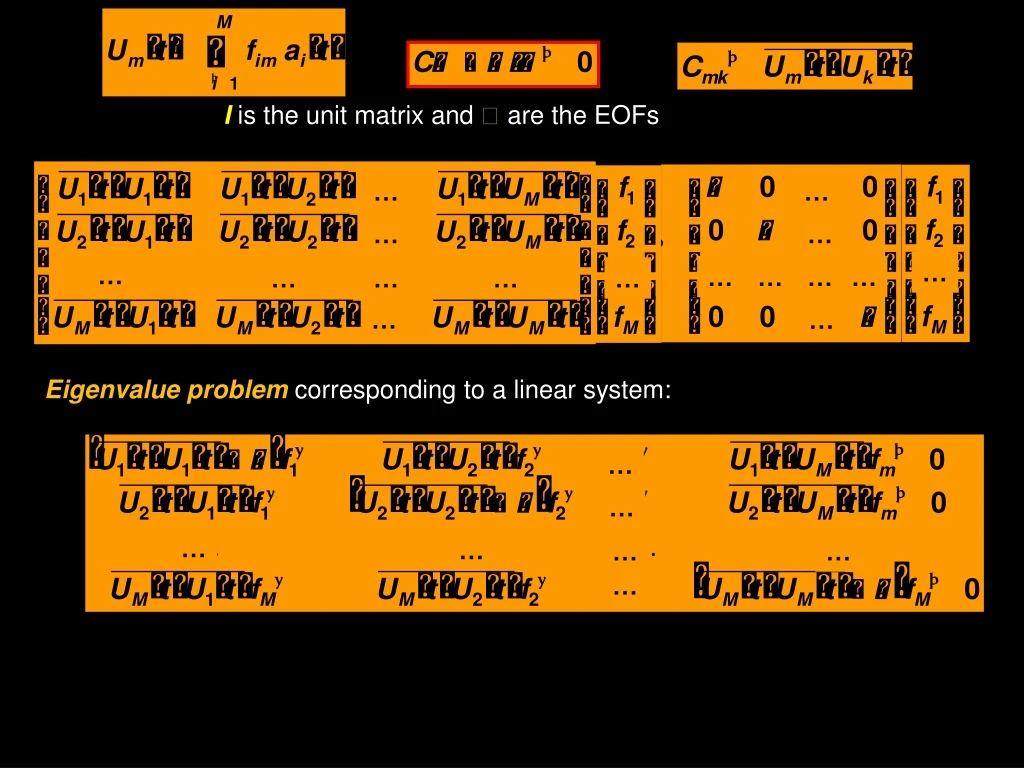
I is the unit matrix and are the EOFs … … … … … … … … … … … … … … … … Eigenvalue problemcorresponding to a linear system: … … … … … … …
Sometimes use another complex form of EOFS. Apply the Hilbert Transformof U to understand a bit more about the phase of propagationof the phenomenon In essence, the Hilbert transform of a signal (time series) produces a complex variable with real part identical to the time series and the imaginary part is shifted 90º from the original (sometimes called the analytical signal): >> t=[1:1:1000]; >> u1=sin(2*pi*t/200); >> plot(t,u1,’LineWidth’,3) u1 t
>> t=[1:1:1000]; >> u1=sin(2*pi*t/200); >> plot(t,u1,’LineWidth’,3) >> >> u2=hilbert(u1); >> hold on; >> plot(real(u2),'r--','LineWidth',3) u t
>> t=[1:1:1000]; >> u1=sin(2*pi*t/200); >> plot(t,u1,’LineWidth’,3) >> >> u2=hilbert(u1); >> hold on >> plot(real(u2),'r--','LineWidth',3) >> plot(imag(u2),'g','LineWidth',3) u t
Hilbert Transformof U can be regarded as the convolution of U with h(t) P is the Cauchy principal value (assigns values to improper integrals) • hilbert uses a four-step algorithm: • 1. It calculates the FFT of the input sequence, storing the result in a vector x. • 2. It creates a vector h whose elements h(i) have the values: • 1 for i = 1, (n/2)+1 • 2 for i = 2, 3, ... , (n/2) • 0 for i= (n/2)+2, ... , n • 3. It calculates the element-wise product of x and h. • 4. It calculates the inverse FFT of the sequence obtained in step 3 and returns the first n elements of the result.
Mean Profile 10 log (echo) b=10*log10(b); bm=mean(b');
Anomaly from Mean b=10*log10(b); ba=b-bm;
REAL EOFs [v,d]=eig(cov(ba’)); plot(v(:,1),z,'LineWidth',3) hold on plot(v(:,2),z,'r','LineWidth',3) plot(v(:,3),z,'g','LineWidth',3) 18% 60% 9%
REAL EOFs Mode 1 = 60% Mode 2 = 18% Mode 3 = 9% ts=ba’*v; plot(ts(:,1),'LineWidth',3) hold on plot(ts(:,2),'r','LineWidth',2) plot(ts(:,3),'g','LineWidth',1)
Hilbert EOF 18% 6% 64% [v,d]=eig(cov(hilbert((ba’))); plot(abs(v(:,1)),z,'LineWidth',3) hold on plot(abs(v(:,2)),z,'r','LineWidth',3) plot(abs(v(:,3)),z,'g','LineWidth',3)
Phase Hilbert EOF Mode 3 = 6% plot(angle(v(:,1))/pi,z,'+','LineWidth',3) hold on plot(angle(v(:,2))/pi,z,'*r','LineWidth',3) plot(angle(v(:,3))/pi,z,'*g','LineWidth',3) xlabel('Mode Phase (rad/\pi)'); ylabel('Depth (m)'); Mode 2 = 18% Mode 1 = 64% Mode Phase
Magnitude of Hilbert EOFs plot(abs(ts(:,1)),'LineWidth',3); hold on plot(abs(ts(:,2)),'r','LineWidth',2) plot(abs(ts(:,3)),'g','LineWidth',1) axis([0 nt 0 6]); xlabel('Time (h)'); ylabel('Mode scale - ABS');
Modes 1 + 2 Real forkeof=1:neof t(keof,:,:)=ts(:,keof)*v(:,keof)'; end Modes 1 + 2 Hilbert Original
6 Modes Real 6 Modes Hilbert Original


