Download
1 / 21
230 likes | 561 Views
FTLE and LCS. Pranav Mantini. Contents. Introduction Visualization Lagrangian Coherent Structures Finite-Time Lyapunov Exponent Fields Example Future Plan. Time-Varying Vector Fields. Vector Field defines a vector( v(x) ) at every point x on the grid

E N D
FTLE and LCS PranavMantini
Contents • Introduction • Visualization • Lagrangian Coherent Structures • Finite-Time Lyapunov Exponent Fields • Example • Future Plan
Time-Varying Vector Fields • Vector Field defines a vector(v(x)) at every point x on the grid • In time variant vector field the vector defined at the points on the grid change with time(v(x,t)). • Creating complex patterns and requires sophisticated techniques for analysis and visualization
Applications • Deepwater Horizon Oil Spill • Thorough analysis of flows plays an important role in many different processes, • Airplane • Car design • Environmental research • And medicine
Mathematical Framework • A time-varying vector field is a map • Satisfies the conditions • ) =
Visualization • Traditionally visualized using Vector Field Topology. • Gives a simplified representation of a vector field a dynamical system, with respect to the regions of different behavior. • VFT deals with the detection, classification and global analysis of critical points • VFT are significantly helpful for visualizing the time independent vector fields.
Visualization • In time varying vector fields, pathlinediverge from stream lines and the critical points move. • Forces to visualize only at a single point of time. • Coherent structures provide a more meaningful representation
LagrangianCoherent Structures • LCS has gained attention in visualizing time dependent vector fields • A set of LCS can represents regions that exhibits similar behavior • example, a recirculation region can be delimited from the overall flow and can represent an isolated LCS • LCS boundaries can be obtained by computing height ridges of the finite-time Lyapunovexponent fields
Real World Correspondence Glaciers Confluences from: www.publicaffairs.water.ca.gov/swp/swptoday.cfm from: www.scienceclarified.com/Ga-He/Glacier.html LCS = Interfaces LCS = Moraines
Finite-Time LyapunovExponent Fields • Scalar Value • Quantifies the amount of stretching between two particles flowing for a given time • High FTLE values correspond to particles that diverge faster than other particles in the flow field High FTLE Values
Finite-Time Lyapunov Exponent Fields • Advect each sample point at time with the flow for time , resulting in a flow map • maps a sample point x to its advection position
Finite-Time Lyapunov Exponent Fields • Give an arbitrary point • Aim of the FTLE is to estimate the maximal growth of during the time period + L2 Norm on both sides =
Finite-Time Lyapunov Exponent Fields • Maximum value can be computed from • maximum stretching would then be the square root of the largest eigenvalue of • FTLE is calculated as
Lagrangian Coherent Structures • Ridge lines in these fields correspond to LCS • Height ridges are locations where a scalar field has a local extremum in at least one direction • Ridge criterion can be formulated using the gradient and the Hessian of the scalar field • Eigenvectors belonging to the largest eigenvalues of the Hessian point along the ridge, and the smallest point orthogonal to the ridge.
Example • Velocity Field • Time-dependent double gyre • Domain [0, 2] x [0, 1]
FTLE and LCS • FTLE • FTLE LCS
Crowd Flow Segmentation & Stability Analysis • (CVPR), 2007
Future Plan • It is obvious that the LCS are influenced by the 3D geometry. • It might be interesting to see how the change in geometry influences the LCS Build Vector Field, Find LCS Change Geometry Estimate LCS
Future Plan • Week – 1&2: Estimate LCS for an example Vector Field • Week – 3: Build a Vector Field from real world scenario • Week – 4: Estimate LCS • Week – 5….: Try to estimate LCS based on geometry and other information, in the absence of a vector field
References • “Visualizing Lagrangian Coherent Structures and Comparison to Vector Field Topology” FilipSadlo and Ronald Peikert Computer Graphics Laboratory, Computer Science Department • Efficient Computation and Visualization of Coherent Structures in Fluid Flow Application.Christoph Garth, Florian Gerhardt, Xavier Tricoche, Hans Hagens • http://mmae.iit.edu/shadden/LCS-tutorial/
Any Questions