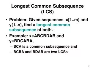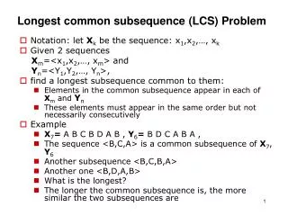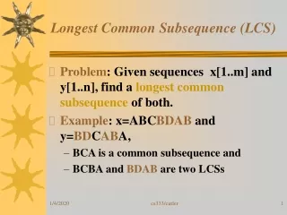
Sparse LCS Common Substring Alignment
This paper presents a novel approach to common substring alignment based on the Longest Common Subsequence (LCS) similarity metric. We introduce a preprocessing stage that constructs a data structure for fast comparisons and an efficient alignment process that significantly reduces computational redundancy. By leveraging the sparsity of LCS, we propose a structured methodology to find the similarity of input strings with a target string, focusing on its application in molecular biology for searching similar sequences. The algorithm reduces time complexity, paving the way for advanced analysis in biological data.


Sparse LCS Common Substring Alignment
E N D
Presentation Transcript
Sparse LCS Common Substring Alignment Gad M .Landau, Baruch Schieber and Michal Ziv-Ukelson CPM03 張耿豪 王姵瑾 吳亭範
Outline • Introduction • Preliminaries • The algorithm • Totally Monotone Rectangular Matrix • Conclusions and Open Problems
Input: a set of strings S1, S2, …, Scand a target string T Output: the similarity of all strings Si with T Under LCS similarity metric Ex: S1=ababaa S2=aabbb T=abab Sim(S1, T) = 4 Sim(S2, T) = 3 Common Substring Alignment
Application • Molecular biology… • Search the most similar strings in database
Main idea • Y is the common substring of Si • Don’t compute of the similarity between Y and T over and over again. • The sparsity of LCS
B C B A D B D B B B O5 3 O4 2 O8 4 I0 0 I1 1 I2 1 I3 1 I5 1 I4 1 I7 1 I6 1 I8 1 O7 4 O6 4 O0 0 O1 1 O2 1 O3 2 D B B T DP Graph Varies by Si Bi G Y Si Speed up Fi Same structure
Three stages • In Common Substring Alignment • Preprocessing stage • Encoding stage • Alignment stage
Preprocessing stage • Parsed for the optimal common substring… compromise • Si = Bi Y Fi T = “BCBADBDCD” Y= “BCBD” S1= “BC BCBD C” B1= “BC” F1 = “C” S2= “E BCBD DBCBD A” B2a = “E” F2a= “DBCBDA” B2b = “EBCBDD” F2b=“A”
In this paper • We assume that Y is given. We focus on the following two stages.
A data structure is constructed which encodes the comparison of Y with T Goal: to speed up alignment stage T B C B A D B D B Bi B I0 0 I1 1 I2 1 I3 1 I4 1 I5 1 I6 1 I7 1 I8 1 G B Y D B O0 0 O1 1 O2 1 O3 2 O8 4 O4 2 O5 3 O6 4 O7 4 Fi B Encoding Stage
Align between Si and T Use the pre-compiled data-structure to align Y and T T B C B A D B D B Bi B I0 0 I1 1 I2 1 I3 1 I4 1 I5 1 I6 1 I7 1 I8 1 G B Y D B O0 0 O1 1 O2 1 O3 2 O8 4 O4 2 O5 3 O6 4 O7 4 Fi B Alignment Stage
Notation • n = |Si| = |T| • L = max{LCS[T, Si]} • Ly=|LCS[T, Y]| • (Ly ≤ |Y|, Ly ≤ L, L ≤ n)
Previous result Encoding stage O(n2+n|Y|) Alignment stage O(n) (SIAM 2001) In this paper Encoding stage O(nLy) Alignment stage O(L) Results Sparcity of LCS: Ly << |Y|, L << n
I0 0 I1 1 I2 1 I3 1 I4 1 I5 1 I6 1 I7 1 I8 1 T B Y D G B O0 O1 O2 O3 O8 O4 O5 O6 O7 Our goal now ?
Auz= substring of A from index u to z, 1≤u≤z≤n I[j]=|LCS[T1j, Bi]| (0,0) 到input row I 的第j個vertex的optimal path‘s weight O[j]=|LCS[T1j, BiY]| B C B A D B D B Bi B I0 0 I1 1 I2 1 I3 1 I4 1 I5 1 I6 1 I7 1 I8 1 B Y D B O0 0 O1 1 O2 1 O3 2 O8 4 O4 2 O5 3 O6 4 O7 4 Fi B DP Graph G
In a given row in the DP graph,LCS has two properties 遞增 每一步頂多增加1 增加一個match B D B A D B D C B C B 2 2 2 1 1 1 1 1 0 Observation
I[j]=|LCS[T1j, Bi]| (0,0) 到input row I 的第j個vertex的optimal path‘s weight O[j]=|LCS[T1j, BiY]| For k = 0,…,L PI[k] Row I 中, weight k 的block的起始index 由DP graph中(0,0)到 row I,weight為k且最左邊的path PO[k] Row O 中, weight k 的block的起始index 由DP graph中(0,0)到 row O,weight為k且最左邊的path Some alternative…
PI[k] and PO[k] are sufficient to represent I[j] and O[j] T I0 0 I1 1 I2 1 I3 1 I4 1 I5 1 I6 1 I7 1 I8 1 G B Y D B O0 0 O1 1 O2 1 O3 2 O8 4 O4 2 O5 3 O6 4 O7 4 Therefore… PI = 0 1 PO = 0 1 3 5 6
Claim • Only the positions PI[r] are sufficient for computing PO[k], r, k = 0,…,L Row I中, 不是PI[r]的index在Row O所能達到的結果,PI[r’]也能達到,甚至更好 • Proof • i1 = PI[k], i3=PI[k+1] if defined • For any index i2, i1<i2<i3 (I[i1]=I[i2]), 對Row O的index j I[i1]+|LCS[Ti1+1j,Y]| ≥ I[i2]+|LCS[Ti2+1j,Y]| (通過i1所走的path至少比通過i2所走的path好)
Given vector PI, compute vector PO! B Y D B Objective now!! T PI = 0 1 ? PO
Observation • When compute PO[k], only PI[r] are candidates, 0≤r≤k • 只有通過row I weight≤k的 path才有可能造成row O的k-path
The Algorithm Encoding Stage Alignment Stage 消消樂 另一半 最近邊界 Total Monotone in O(n) S in O(n|LCS(Y,T)|) Construct LEFT in O(n) Column Minima of LEFT in O(n)
PI 0 1 2 Bi Y Fi PO 0 1 2 3 4 B C B A D B D C 0 B A B D B
T PI[r] j Bi r PI[r] PI k-r = LCS[TjPI[r]+1,Y] Y PO PO[k] Fi
r r+1 r-1 PI[r] PI[r+1] PI[r-1] k-r-1 k-r k-r+1 PO[k]=? PO[k]=? PO[k]=? T Find Optimal SubPath Bi PI Y PO Fi
r r+1 r-1 PI[r] PI[r+1] PI[r-1] k-r-1 k-r k-r+1 PO[k]=? PO[k]=? PO[k]=? Encoding Stage • Preprocessing: Si unknown • Table S: alignment of T, Y Bi PI Y PO Fi S[i, w] = min{j | |LCS[Tji+1, Y]| = w}
Algorithm S[i, w] = min{j | |LCS[Tji+1, Y]| = w} for i = 0 to |T| S[i, 0] i for k = 0 to … S[i, k+1] = S[i, k] + d next k next i
起點 weight Observation S[1,0] = 1 S[1,1] = S[1,0] + 最近邊界距離* = 1 + 1 S[1,2] = S[1,1] + 最近邊界距離* = 2 +2 =4 • S[i, k+1] = S[i, k] + d T C B A D B D C B B A Y B D B 1 2 3 4 5 6 7 8 9
尋找最近邊界 • O( |Alphabet| * (|Y|+|T|) ) preprocessing • O(1) finding next
Preprocessing • Finding all matches • foreach alphabet, scan Y, T for position • matches 現(B in Y) cross 現(B in T) • construct a fastfind structure T C B A D B D C B B A Y B D B
Algorithm S[i, w] = min{j | |LCS[Tji+1, Y]| = w} for i = 0 to |T| S[i, 0] i for k = 0 to O(|LCS(Y,T)|) S[i, k+1] = S[i, k] + d next k next i
i The Inner Loop—O(|LCS(Y,T)|) T B C B A D B D C B A Y B D B S[i, k+1] = S[i, k] + d
Complexity • Assume |T| > |Y| • preprocessing O( |Alphabet| * (|Y|+|T|) ) • The inner loopO( |LCS(Y,T)| ) • The outter loopO(|T|) • OverallO( |T|*|LCS(Y,T)| ) for i = 0 to |T| S[i, 0] i for k = 0 to O(|LCS(Y,T)|) S[i, k+1] = S[i, k] + d next k next i
The Algorithm Encoding Stage Alignment Stage 消消樂 另一半 最近邊界 S in O(n|LCS(Y,T)|) Construct LEFT in O(n) Column Minima of LEFT in O(n)
r r+1 r-1 PI[r] PI[r+1] PI[r-1] k-r-1 k-r k-r+1 PO[k]=? PO[k]=? PO[k]=? Alignment Stage PO[k] = minkr=0{ S[ PI[r], k-r] } T Bi PI Y PO Fi
Construction of Left(1) PO[k] = minkr=0{ S[ PI[r], k-r] }
Construction of Left(2) PO[k] = min{ }
Construction of Left(3) PO[L]=min{} PO[0]=min{} PO[1]=min{}
Undefined Region in LEFT[][] PI[r+1] PI[r-1] PI[r] PI k-r-1 k-r k-r+1 PO PO[k]=? PO[k]=? PO[k]=? S[i, w] = min{j | |LCS[Tji+1, Y]| = w} 起點 增加的weight PO[L]=min{} PO[0]=min{} PO[1]=min{}
Good Property of Left[][] • Totally Monotone Rectangular Matrix Convex Concave Or
Reduced Problem • The minimum value of each column • nxn total monotone matrix O(n)
Find Column Minima Recursively Minima(Am×n) Bn×n消(Am×n) If #row(Bn×n) = 1 return the positions of minima 另一半by Minima(半(B)) return the positions of minima
半 消 半 消 半 消
The Algorithm Encoding Stage Alignment Stage 消消樂 另一半 最近邊界 S in O(n|LCS(Y,T)|) Construct LEFT in O(n) Column Minima of LEFT in O(n)
≤ 消::m×n n×n n Type A: 自亂陣腳 Type B: 全排覆沒 ≤ ≤ m >
消 at the n-th row n Type C: 敵前投降 m ≤
Complexity of 消—O(m) • At most m-n deletions • B全排覆沒+C敵前投降 = O(m-n) • 最左走到n • A自亂陣腳-B全排覆沒 = O(n) • A+B+C = (A-B)+2(B+C) = O(n+2*(m-n)) = O(2m – n) = O(m)
The Algorithm Encoding Stage Alignment Stage 消消樂 另一半 最近邊界 S in O(n|LCS(Y,T)|) Construct LEFT in O(n) Column Minima of LEFT in O(n)
Find Column Minima Recursively Minima(Am×n) Bn×n消(Am×n) If #row(Bn×n) = 1 return the positions of minima 另一半by Minima(半(B)) return the positions of minima