Eng. 6002 Ship Structures 1
Eng. 6002 Ship Structures 1. Matrix Analysis Using MATLAB Example. Introduction. Last class we divided the FEM into five steps: construction of the element stiffness matrix in local coordinates, transformation of the element stiffness matrix into global coorindinates,

Eng. 6002 Ship Structures 1
E N D
Presentation Transcript
Eng. 6002 Ship Structures 1 Matrix Analysis Using MATLAB Example
Introduction • Last class we divided the FEM into five steps: • construction of the element stiffness matrix in local coordinates, • transformation of the element stiffness matrix into global coorindinates, • assembly to the global stiffness matrix using transformed element stiffness matrices, • application of the constraints to reduce the global stiffness matrix, • determination of unknown nodal displacements.
The Method • The stiffness matrix for each element is
The Method • this matrix describes the stiffness of an elastic element that relates the load vector to the displacement vector
The Method • the element stiffness matrix transformed to global coordinates is defined as:
The Method • The transformation matrix is given by:
Example cont. • In order to easily combine the element stiffness matrices, each element stiffness matrix is stored in a matrix the size of the global stiffness matrix, with the extra spaces filled with zeros. • In this example, the element stiffness matrix for element 1 is stored in the portion of the global stiffness matrix that involves nodes 1 and 2, • i.e., the upper 6 x 6 portion of the matrix. Thus, the expanded stiffness matrix that describes element 1 is given by:
Example cont. • The element stiffness matrix for element 2 is stored in the portion of the global stiffness matrix that involves nodes 2 and 3, i.e., the lower 6 x 6 portion of the matrix. The expanded stiffness matrix that describes element 2 is given by:
Example cont. • The expanded individual stiffness matrices can now be added together so that the global stiffness matrix for the two-element structure is given as:
Next Class Example 1: two beam elements • A simple structure made of two beams has the following parameters • L1 = 12 in, L2 = 18 in, and E = 30 x 106 psi. The cross-section of the beams are 0.5 in x 0.5 in and θ = 45°. If a downward vertical force of 1000 lb is applied at node 2, find the displacement at node 2.
Step 1 • The first step in the solution procedure is to discretize the domain, i.e. select the number of elements. As a first approximation, the problem is modeled with two beam elements. The element stiffness matrix for each of the beam elements is of the form:
Step 1 (code) • m = 2; % number of elements • b = [0.5 0.5]; % width (in) • h = [0.5 0.5]; % height (in) • a = b.*h; % cross-sectional area • I = b.*h.^3./12; % moment of inertia • l = [12 18]; % length of each element (in) • e = [30*10^6 30*10^6]; % modulus of elasticity (psi) • theta = [0 -45*pi/180]; % orientation angle • f = -1000; % force (lbs) • % • % Step 1: Construct element stiffness matrices • % • k = zeros(6,6,m); • for n = 1:m • k11 = a(n)*e(n)/l(n); k22 = 12*e(n)*I(n)/l(n)^3; • k23 = 6*e(n)*I(n)/l(n)^2; k33= 4*e(n)*I(n)/l(n); • k36 = 2*e(n)*I(n)/l(n); • k(:,:,n) = [k11 0 0 -k11 0 0;0 k22 k23 0 -k22 k23;0 k23 k33 0 -k23 k36;-k11 0 0 k11 0 0;0 -k22 -k23 0 k22 -k23; 0 k23 k36 0 -k23 k33]; • end
Step 1 • Note: we are building 3D matrices (i.e. a series of 2D matrices – with size=m) • See k in code
Step 2 • The second step is to transform each element stiffness matrix in local coordinates to the global coordinate system. • This transformation is accomplished by . • The transformation angle for element 1 is θ = 0, and, thus, the transformation matrix is simply the identity matrix. Because the rotation angle is measured counterclockwise, the transformation angle for element 2 is θ = -45°.
Step 2 • for n = 1:m • c = cos(theta(n)); s = sin(theta(n)); • lamda = [c s 0 0 0 0; -s c 0 0 0 0; 0 0 1 0 0 0; 0 0 0 c s 0; 0 0 0 -s c 0; 0 0 0 0 0 1]; • kbar (:,:,n) = lamda'*k(:,:,n)*lamda;
Step 3 • The third step is to assemble the global stiffness matrix that describes the entire structure by properly combining the individual element stiffness matrices. • Elements stiffness matrices are stored in the proper portion of the matrix, i.e. each matrix is shifted by three rows and three columns.
Step 3 • % Step 3: Combine element stiffness matrices to form global stiffness matrix • % • for i = 1:6 • for j = 1:6 • Ke(i+shift,j+shift,n) = kbar(i,j,n); • end • end • shift = shift + 3;
Step 3 • We then add the matrices together to form the global stiffness matrix • K = sum(Ke,3)
Step 4 • The fourth step is to apply the constraints and reduce the global stiffness matrix so that the specific problem of interest can be solved. For this problem, the displacements at node 1 and node 3 are known, i.e. U1 = U2 = U3 = U7 = U8 = U9 = 0, and the loads are applied to node 2 are specified, i.e. F4 = 0, F5 = -1000 lb, and F6 = 0. Thus, the system of equations can be written as:
Step 4 • This problem has three unknowns, U4, U5, and U6, and, thus, requires three independent equations. • Matrix algebra allows three independent equations to be constructed by the removal of the rows and columns that correspond to the known displacements, i.e. the global stiffness matrix reduces to:
Step 4 the stiffness matrix reduces to:
Step 4 • Step 4: Reduce global stiffness matrix with constraints • % • Kr = K; • Kr(:,9) = []; Kr(9,:) = []; Kr(:,8) = []; Kr(8,:) = []; • Kr(:,7) = []; Kr(7,:) = []; • Kr(:,3) = []; Kr(3,:) = []; Kr(:,2) = []; Kr(2,:) = []; • Kr(:,1) = []; Kr(1,:) = []
Step 4 • The numerical values from the code
Step 5 • The final step is simply to solve the reduced system of equations for the unknown displacements. • Fr = [0; f; 0]; • Ur = Kr\Fr • The numerical solution from the MATLAB code is • U4 = -0.0016 in, • U5 = -0.0064 in, and • U6 = -0.0003 radians.
Discussion • This problem is statically indeterminate, and the solution is not trivial. • Additional information can be found with the addition of nodes. For example, the deflection at the midpoint of each element can be found if two additional nodes are added. • Of course, then a 9 x 9 system of equations must be solved. Note that the addition of nodes at the midpoints does not change the solution at node 2.
Assignment • Using the approach outlined in this lecture, develop a matlab routine to find the deflection at the midpoint of each element shown. • L1 = 12 in, L2 = 18 in, and E = 30 x 106 psi. The cross-section of the beams are 0.5 in x 0.5 in and θ = 45°. If a downward vertical force of 1000 lb is applied at node 2