Chapter 3 Multiple Linear Regression
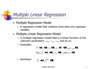
Chapter 3 Multiple Linear Regression. 3.1 Multiple Regression Models. Suppose that the yield in pounds of conversion in a chemical process depends on temperature and the catalyst concentration. A multiple regression model that might describe this relationship is

Chapter 3 Multiple Linear Regression
E N D
Presentation Transcript
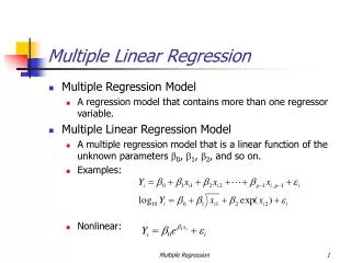
3.1 Multiple Regression Models • Suppose that the yield in pounds of conversion in a chemical process depends on temperature and the catalyst concentration. A multiple regression model that might describe this relationship is • This is a multiple linear regression model in two variables.
3.1 Multiple Regression Models Figure 3.1 (a) The regression plane for the model E(y)=50+10x1+7x2. (b) The contour plot.
3.1 Multiple Regression Models In general, the multiple linear regression model with k regressors is
3.1 Multiple Regression Models Linear regression models may also contain interaction effects: If we let x3 = x1x2 and 3 = 12, then the model can be written in the form
3.2 Estimation of the Model Parameters 3.2.1 Least Squares Estimation of the Regression Coefficients Notation n – number of observations available k – number of regressor variables, p-- k+1( number of regression coefficients) y – response or dependent variable xij – ith observation on jth regressor j.
3.2.1 Least Squares Estimation of the Regression Coefficients The sample regression model can be written as
3.2.1 Least Squares Estimation of the Regression Coefficients The least squares function is The function S must be minimized with respect to the coefficients.
3.2.1 Least Squares Estimation of the Regression Coefficients The least squares estimates of the coefficients must satisfy
3.2.1 Least Squares Estimation of the Regression Coefficients Simplifying, we obtain the least squares normal equations: The ordinary least squares estimators are the solutions to the normal equations.
3.2.1 Least Squares Estimation of the Regression Coefficients Matrix notation is more convenient to find the estimiates Let where
3.2.1 Least Squares Estimation of the Regression Coefficients
3.2.1 Least Squares Estimation of the Regression Coefficients These are the least-squares normal equations. The solution is
3.2.1 Least Squares Estimation of the Regression Coefficients Linear Regression Analysis 5E Montgomery, Peck & Vining
3.2.1 Least Squares Estimation of the Regression Coefficients The n residuals can be written in matrix form as There will be some situations where an alternative form will prove useful Where H is called hat matrix
Example 3-1. The Delivery Time Data The model of interest is y = 0 + 1x1+ 2x2 +
Example 3-1. The Delivery Time Data Figure 3.4Scatterplot matrix for the delivery time data from Example 3.1. R codes for the figure in “Chapter_3_nulti_reg.txt”
Example 3-1 The Delivery Time Data Figure 3.5Three-dimensional scatterplot of the delivery time data from Example 3.1.
3.2.3 Properties of Least-Squares Estimators • Statistical Properties • Variances/Covariances p×p matrixDiagonal entities Cjj are variances, And the remaining Cij are covariance of two regression coefficients
3.2.4 Estimation of 2 • The residual sum of squares can be shown to be: • The residual mean square for the model with p parameters is: Linear Regression Analysis 5E Montgomery, Peck & Vining
3.2.4 Estimation of 2 • Recall that the estimator of 2 is modeldependent - that is, change the form of the model and the estimate of 2 will invariably change. • Note that the variance estimate is a function of the errors; “unexplained noise about the fitted regression line” Linear Regression Analysis 5E Montgomery, Peck & Vining
Which model is better? • Let’s calculate the variance of errors of different models Model 1; consider two reggressors ( case and distance) Model 2; only consider reggressor “case” We would usually prefer a model with a small residual mean square (estimated variance of error).
Example 3.2 Delivery Time Data Linear Regression Analysis 5E Montgomery, Peck & Vining
Example 3.2 Delivery Time Data Linear Regression Analysis 5E Montgomery, Peck & Vining
3.2.5 Inadequacy of Scatter Diagrams in Multiple Regression • Scatter diagrams of the regressor variable(s) against the response may be of little value in multiple regression. • These plots can actually be misleading • If there is an interdependency between two or more regressor variables, the true relationship between xi and y may be masked. Linear Regression Analysis 5E Montgomery, Peck & Vining
Illustration of the Inadequacy of Scatter Diagrams in Multiple Regression
Scatterplot is useful if… • There is only one (of few) dominate reggressor • The regressors operate nearly independent • !!! Scartterplot could be misleading when several important regressors are related. ( we will discuss the analytical methods for sorting out the relationships between regressors in later chapter.
3.3 Hypothesis Testing in Multiple Linear Regression Once we have estimated the parameters in the model, we face two immediate questions: 1. What is the overall adequacy of the model? 2. Which specific regressors seem important?
3.3 Hypothesis Testing in Multiple Linear Regression Next we will consider: • Test for Significance of Regression (sometimes called the global test of model adequacy) • Tests on Individual Regression Coefficients (or groups of coefficients) Linear Regression Analysis 5E Montgomery, Peck & Vining
3.3.1 Test for Significance of Regression • The test for significance is a test to determine if there is a linear relationship between the response and any of the regressor variables • The hypotheses are H0: 1 = 2 = …= k = 0 H1: j 0 for at least one j Linear Regression Analysis 5E Montgomery, Peck & Vining
3.3.1 Test for Significance of Regression • As in Chapter 2, the total sum of squares can be partitioned in two parts: SST = SSR + SSRes • This leads to an ANOVA procedure with the test(F) statistic
3.3.1 Test for Significance of Regression • The standard ANOVA is conducted with
3.3.1 Test for Significance of Regression ANOVA Table: or p-1 or n-p Reject H0 if Linear Regression Analysis 5E Montgomery, Peck & Vining
3.3.1 Test for Significance of Regression • R2 • R2 is calculated exactly as in simple linear regression • R2 can be inflated simply by adding more terms to the model (even insignificant terms) • Adjusted R2 • Penalizes you for added terms to the model that are not significant
Example 3.3 Delivery Time Data Linear Regression Analysis 5E Montgomery, Peck & Vining
Example 3.3 Delivery Time Data To test H0: 1 = 2 = 0, we calculate the F–statistic: Linear Regression Analysis 5E Montgomery, Peck & Vining
Example 3.3 Delivery Time Data R2 = 0.9596 Adjusted R2 = 0.9559 To look at the overall significance of regression:p-value of F test R2 Adjusted R2
Adding a variable will always result in increase of R –squared. Our goal is to only add necessary regressors that will reduce the residual variability.. But we do not want over-fitting( add un necessary variables ( will learn variable selection procedure in later chapters).
3.3.2 Tests on Individual Regression Coefficients • Hypothesis test on any single regression coefficient: • Test Statistic: • Reject H0 if |t0| > • This is a partialor marginaltest!
The Extra Sum of Squares method can also be used to test hypotheses on individual model parameters or groups of parameters Full model Linear Regression Analysis 5E Montgomery, Peck & Vining

