Download

1 / 40
420 likes | 640 Views
CFA Review 3 Modern Portfolio Theory, Asset Pricing and Portfolio Evaluation. policy statement. TOTAL RETURN= INCOME YIELD + CAPITAL GAIN YIELD Objectives – Think in terms of risk and return to find the “best” weights—i.e.,

E N D
CFA Review 3Modern Portfolio Theory, Asset Pricing and Portfolio Evaluation
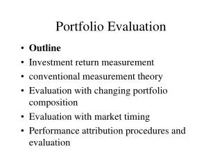
policy statement • TOTAL RETURN= INCOME YIELD + CAPITAL GAIN YIELD • Objectives – Think in terms of risk and return to find the “best” weights—i.e., • Capital preservation (high income, low capital gain) Low to moderate risk • Balanced return (Balanced capital gains and income reinvestment)moderate to high risk • Pure Capital appreciation (high capital gains, low to no income)High risk • Constraints - liquidity, time horizon, tax factors, legal and regulatory constraints, and unique needs and preferences • Management - Define an allowable allocation ranges based on policy weights • Selection - Define guideline to pick securities to purchase for the portfolio (optional)
Measuring Returns • r=FV/PV-1 or r=ln(FV/PV) • When you have many returns: • Arithmetic mean (R=1/n x Sri)--2 weaknesses, 1) extreme values effect, 2)# of observation need to be known • Historical (R=1/n x Srt)-- • Cross-sectional (R=1/n x Sri) or Probability weighted (R=Spiri) • Geometric mean(R=[P(1+ri)]1/n -1) • Historical (R=[P(1+rt)]1/n -1) • Cross-sectional (R=[P(1+ri)]1/n -1) • Example 1: 3 returns (10%, 12%, 14%) • AM =(10%+12%+14%)/3=12% • GM =[(1+10%)x(1+12%)x(1+14%)]1/3-1=11.988% • Example 2:
Measuring Risk Standard deviation of returns with equally weighted deviations: Standard deviation of returns with unequally weighted deviations: Standard deviation of unequally weighted standard deviations:
Example 3: A .10 .07 B .20 .1
Portfolio Risk-Return Plots for Different Weights E(R) Rij = -0.50 f Rij = -1.00 B g h i j Rij = +1.00 k Rij = +0.50 A Rij = 0.00 With perfectly negatively correlated assets it is possible to create a two asset portfolio with almost no risk Standard Deviation of Return
The Capital Market Line (CML) • Imagine two portfolio: (1) a COMPLETELY DIVERSIFIED risky portfolio with an expected return of Rm and a standard deviation of σm and (2) a riskless portfolio of t-bills with an expected of Rf and a standard deviation close to zero. • You allocate Wrf in the riskless portfolio and (1-Wrf) in the risky (best of the best portfolio) • The standard deviation and expected return of this portfolio shall be: σp=(1-Wrf) x σm or Wrf=1- σp/σm, then Rp=Wrf x Rf + (1-Wrf) x Rp replace Wrf by 1- σp/σm RP= Rf + (Rm –Rf) /σm x σp Capital Market Line (CML) Rp= intercept + slope x σp
CML and leverage How is the concept of leverage included in the CML? Wrf>0 less risk; Wrf<0 more risk • Notice that the decision to invest has been separated from the decision to select specific investments (separation theorem). In a CML world, you do not worry about “what to invest in since all investors will buy the same portfolio (M)—i.e., the investment selection process has been simplified from stock analysis and picking to efficient portfolio construction through diversification! Wrf>0 Wrf<0 Wrf=0 Where, Wrf=1-(sP/sM)
Utility Value of an Investment There is a trade off between risk and return and “intelligent” investors like more returns and less risk. An investor is indifferent of the trade-off between risk and return at each indifference curve. However investors like I2 better than I1. Combining utility curves and CML, the optimal portfolio for each investor is the highest indifference that is tangent to the CML. Risk aversion refers to the fact that investors prefer less risk than more risk. Utility is often described in a quadratic format: Up=Rp-0.5 x Rz x sp2 Where Up is an investor’s utility for holding portfolio p Rp is the expected return of portfolio p Rz is the risk aversion value sp2 is the variance of portfolio p More preferred direction for indifference curves Example 4: Joe L’Outre has a risk aversion value of 4, which of portfolios A, B, and C is best for him?
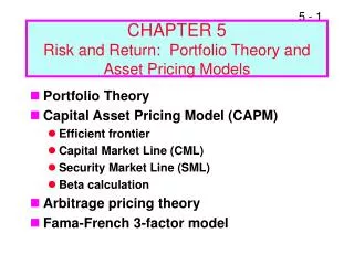
Risk and Diversification Return = expected + unexpected Risk (return)= 0 + market risk + business risk Risk (return)= 0 + Systematic Risk + Non-systematic risk Ri=RF + RRP, then… • Security risk premium = (Ri- RF), Market risk premium = (Rm- RF) • If security risk premium=β x market risk premium • Then, (Ri- RF) =β x (Rm- RF) That is, Ri = RF +β x (Rm - RF)
CAPM Assumptions • Ri = RF +β x (Rm - RF) where b = cov(i,m)/sm2 • 8 underlying assumptions (learn by heart): • All investors use the (Markowitz) mean-varianc eframework to select securities (that is, investors have quadratic utility functions and security returns are normally distributed) • Investors can borrow and lend any amount of money at the risk-free rate • Investors have homogenous expectations (that is, if they look at a stock, they all see the same risk/return distribution) • All investors have a 1-period time horizon • All investments are indefinitely divisible (that is, you can buy/sell fraction of shares of a stock or portfolio • No taxes and no transaction costs • No inflation and interest rates do not change • Capital markets are in equilibrium
CAPM Implications • 4 implications • Because all investors have the same expectations all use mean-variance analysis, they identify the same optimal portfolio and combine it with a risk free asset to create there own portfolio. • Because all investors hold the same risky portfolio, the weight on each asset must equal to the proportion of its market value to the total value of the portfolio. • Since all investors hold the market with some proportion of the risk free asset, the market portfolio must be the point of tangency between the CML and the efficient frontier. • The SML describes the relationship between the expected return and risk of all assets – individual securities and portfolios.
Example 5 RFR = 6% RM = 12% E(RA) = 0.06 + 0.70 (0.12-0.06) = 0.102 = 10.2% E(RB) = 0.06 + 1.00 (0.12-0.06) = 0.120 = 12.0% E(RC) = 0.06 + 1.15 (0.12-0.06) = 0.129 = 12.9% E(RD) = 0.06 + 1.40 (0.12-0.06) = 0.144 = 14.4% E(RE) = 0.06 + -0.30 (0.12-0.06) = 0.042 = 4.2%
Comparison of Required Rate of Return to Estimated Rate of Return
Plot of Estimated Returnson SML Graph .22 .20 .18 .16 .14 .12 Rm .10 .08 .06 .04 .02 C SML A E B D -.40 -.20 .20 .40 .60 .80 1.20 1.40 1.60 1.80
Example 6 • You gather the following information about two stocks A and B, the SP500 and the treasury bill:
What would be the allocation to A and B if you chose the minimum risk portfolio? If Wa=W then Wb=1-W and the variance of the portfolio is
2. Which stock would you consider as an addition to a portfolio made of the SP500? Which stock would you consider for stand-alone portfolio? 2.A Stock to consider as an addition to a portfolio made of the SP500 Get the alpha of each stock—i.e., first get the theoretical (CAPM) return, then subtract it to the expected return. To get CAPM return: Ra=Rf+BETA(A) x (Rm-Rf) Rb=Rf+BETA(B) x (Rm-Rf) Rf is the treasury bill return=2% Rm is the sp500 return=5.5% (it is the weighted average return for sp500) sM=(0.0014749)1/2=3.84% BETA(A)=COV(A,M)/VAR(M)= -0.0037374/ 0.0014749=-2.53 BETA(B)= COV(B,M)/VAR(M)= 0.00865/ 0.0014749=5.85 Then Ra=Rf+BETA(A) x (Rm-Rf)=2%-2.53*3.5%=-6.86% Rb=Rf+BETA(B) x (Rm-Rf)=2%+5.85*3.5%=22.48% ALPHA(A)=7.25%-(-6.86%)=14.11%Undervalued ALPHA(B)=17%-22.48%= -5.48%Overvalued Then you would A to a well-diversified portfolio like A 2.B Stock to consider for stand-alone portfolio get the Coefficient of Variation Calculate the Coefficient of Variation: • CV(A)=9.8%/7.25%=1.35 • CV(B)=23.04%/17%=1.35 • There are basically equivalent in terms of reward to risk in a stand-alone portfolio
3. How much (proportions) would you invest in A and B in order to get a portfolio as risky as the market? The market has a beta of 1; Solve a system of two equations: Wa x BETA(A)+Wb x BETA(B)=1 Wa+Wb=100% Then, Wb=[1-BETA(A)]/[BETA(B)-BETA(A)] BETA(A)=COV(A,M)/VAR(M)= -0.0037374/ 0.0014749=-2.53 BETA(B)= COV(B,M)/VAR(M)= 0.00865/ 0.0014749=5.85 Wb=42% So, Wa=58% 4.You have created your AB portfolio, then you decide to sell A and invest the proceed in T-bills. What the new portfolio Expected return, standard deviation and beta? Wb=42%; Wa=58% sell A, buy TBills Wrf=58% BETA(new portfolio)=Wb x BETA(B) +Wrf x BETA(Rf) and of course BETA(Rf)=0; sRf = 0 • BETA(new portfolio)=.42 x 5.85=2.46 • E(new portfolio)=.42 x 17% + .58 x 2%=8.3% • s (new portfolio)=.42 x 23.04%=9.68% (from the portfolio risk equation with 2 assets, it simplifies a lot as sRf = 0)
Efficient markets • An efficient capital market is one in which the current price fully reflects all the information currently available for the security, including risk. • An informationally efficient capital market is one in which security prices adjust rapidly and completely to new information, which enter the market in a random and unpredictable manner and therefore causes stock prices to change in a random and unpredictable fashion. • Market efficiency is based on the following set of assumptions: • A large number of profit maximizing participants are analyzing and valuing securities independent of each other. • New information comes to the market on a random fashion, and news announcements are independent of each other in regard to timing • Investors adjust price estimates rapidly to reflect their interpretation of the new information received. Market efficiency does not assume that participants adjust prices correctly, just that price adjustments are unbiased. • Expected returns explicitly include risk in the price of the security.
Efficient market hypothesis • Fama divided the efficient market hypothesis into 3 categories: • Weak-form efficient markets: current prices fully reflect all currently available security market information. Thus, past prices and volume information has no predictive power an investor cannot achieve excess return with technical analysis. • Semi-strong efficient markets: current prices rapidly adjust to the arrival of new public information and fully reflect all publicly available information. That is, all security market and non-market publicly available information an investor cannot achieve excess return with fundamental analysis. • Strong form efficient markets: prices fully reflect all information for public and private sources. That is, all market, non-market public, and private (inside) information. There is no such thing as abnormal returns.
Technical Vs. Fundamental analysis • Fundamentalist believes that he can predict futures price patterns by analyzing earnings and other publicly available information (make economic –risk/return--expectations on demand and supply shifts). Fundamentalists believe that price adjustment to new info is rapid. • The technical analyst believes he can predict prices based on historical prices and volume, e.g., price adjustment to new information is slow. A technical analyst believes that prices are determined by supply and demand, which are driven by both rational and irrational behaviors.
Technical Analysis • PRO: Quick, easy, no knowledge of accounting, incorporate psychological with econ reasons behind price changes, and it tells when to buy. • CON: Challenged by ENH, success strategy cannot be repeated, too subjective, no underlying theory, rules change over time, self-fulfilling prophecy leading to prices that say only temporarily. • Dow theory: price moves in trends (major, intermediate, and short-term) • Trading ratio (AKA TRIN)=(adv.issues/decl. issues)/ (adv.vol/decl. vol) –If>1, market overbought; If<1, market oversold • Support and resistance levels: normal rang of price fluctuation – support price is cheap, resistance price is expensive. • Moving average: if stock prices move by trends, then MA lines show these price trends—i.e, if 80% of stocks are above the market 200 MA, the market is considered overvalued. if 20% of stocks are above the market 200 MA, the market is considered undervalued • Relative Strength= stock price/market price. If increasing (decreasing) overtime, stock is overperforming (underperforming). Help differentiate between stock-specific or market (macro) movements.
Tests of EMH • Event studies: • Stock splits: no short-term or long term increase in abnormal returns as a result of a splits. Supports EMH. • IPOs: If investment bankers underprice issues, then abnormal return should occur. Tests show that IPOs are underpriced by 15% (on average), but prices adjust within a day. Supports EMH. • Exchange listing: Does the choice of the exchange increase liquidity and reputation (therefore abnormaly increase long-run value of stock prices)? No. Supports EMH. However, there are short term profit opportunities around the listing date, which do not support EMH. • Accounting changes: Markets react quickly to accounting changes. Supports EMH.
Challenges to EMH • Magnitude issues, selection bias, lucky event and predictability tests • Magnitude issues: large investors (institutional) can influence prices – EMH still stands but the degree of efficiency still varies. • Selection bias: if an investment strategy works, it will not be released to the public. That is, all public strategies have already been tested and proved to fail: EMH cannot be proven using these strategies. • Lucky Event: some investors simply beat the market by getting lucky. On average, there are as many lucky as unlucky investors. • Predictability: Some variables are shown to have predictable properties for stock returns (dividend yield, earnings yield, and bond yield spreads). However, it can be argued that these variables are rather linked to risk than market inefficiency. As for dividend yields and earning yields, lower stock prices will increase both dividend and earning yield and imply a higher risk premium and thus higher expected returns.
Market Anomalies • Earning surprises to predict returns and identify stocks that could earn abnormal returns. • Calendar studies: January anomaly (profit by buying in late December an selling early January); weekend effect (returns for week days are on average positive, and negative from Friday close to Monday open) • PE (low PE stocks have returned more than high PE stocks) • Size: small firm have returned more than large firms • Neglected firms: firms with unusually low number of analysts covering them have higher returns – the excess return is likely attributed to the lack of institutional interest and it affects firms of all sizes. • PB – the greater the book to price ratio (smaller PB), the higher the returns Many of these anomalies are at the origin of extended asset pricing model (extended from CAPM) such as the 3-factor model of Fama and French which includes in addition to the market premium, a size and value premiums.
Behavioral Interpretations and EMH • Overconfidence (when one believes they can better interpret information than the average investor) • Conservatism (underreaction to news events) • Fear of Regret (hold on too long on an investment) • Reference Points (rather than looking at outcomes, profits are estimated as compared to a reference point) • Effects of Past events (take more risk after making money, and less risk after losing money) • Mental Accounting (profit target as a function • Representativeness (purchase past winners, good companies are good stocks)
Other issues affecting EMH • Mutual Fund performance –no significant difference of performance between mutual funds and indexes. Though, few portfolio managers were able to consistently beat the index. In general terms, mutual funds tend to under-perform indices. Performance of funds is also subjected to survivorship bias. • Time Varying Volatility: Volatility responds to news events and future volatility is forecastable using GARCH models. • Equity Premium Puzzle: historically it is around 5% if we use the history of the stock market. However, it has varied significantly – from 1872 to 1949, historical and predicted were similar; from 1950 to 1999, realized returns were higher than predicted.
Portfolio Performance • Measuring returns • Holding period 1 • Beginning price: 100 • Dividends paid : 2 • Ending price: 120 • Holding period 2 (buy 1 more share at the beginning) • Beginning price: 240 (2 shares) • Dividends paid : 4 ($2 per share) • Ending price: 260 (2 shares) • Time weighted returns (method of preference in the industry) • HPR1=(122/100-1)=22% and HPR2=(264/240-1)=10% • Time weighted return = [(1+22%)x(1+10%)]1/2-1=15.84% • Dollar-weighted returns • Solve r: 100+120/(1+r)=2/(1+r)+264/(1+r)1/2 • In calc: cfo=-100; cf1=-118; cf2=264 comp IRR=13.86%
Composite Portfolio Performance Measures • Treynor Measure SML ; T=(Rp-Rf)/β • Sharpe Measure CML; S=(Rp-Rf)/σ • Jensen Measure SML; J=α=(Rp –Rf) – β (Rm – Rf) • Information ratioSML:
Treynor versus Sharpe Measures • Beta vs. Standard Deviation • Treynor –> uses SML, thus focus on Beta assumes that portfolio is well diversified. • Sharpe-> uses the CML, thus focus on standard deviationassumes that portfolio is not well diversified. • Ranking differences from different diversification levels. (SML vs. CML)R2 will tell you! • Benchmark choice may affect the R2 • The Jensen Measure • Requires use of different RFR, Rm, and Rj, for each period. • Assumes portfolio is well diversified and only considers systematic risk. • Provides inferences about abnormal gain/loss • Regression of (Rj- RFR) and (Rm - RFR). • R2 can be useful as a measure of diversification.
The Information Ratio Performance Measure • Appraisal ratio • measures average return in excess of benchmark portfolio divided by the standard deviation of this excess return
M2 • CML uses sp/sm and M2 uses sm/sp ; thus M2 is to be compared to the market return: • If M2>Rm, Portfolio above CML it outperformed the market on a risk adjusted basis • If M2<Rm, Portfolio above CML it underperformed the market on a risk adjusted basis
Potential Bias of One-Parameter Measures • positive relationship between the composite performance measures and the risk involved • alpha can be biased downward for those portfolios designed to limit downside risk • Need to break down performance: • Performance attribution analysis • Market timing ability
Performance Attribution Analysis • Decomposing overall performance into components • Components are related to specific elements of performance: • Asset Allocation • Industry/Sector Allocation • Security Choice Selection • Thus, Contribution for asset and sector/industry allocation + Contribution for security selection = Total Contribution from asset class
Example : PAA Benchmark Manager A Manager B Weight Return Weight Return Weight Return Stock 0.6 -5% 0.5 -4% 0.3 -5% Bonds 0.3 -3.5 0.2 -2.5 0.4 -3.5 Cash 0.1 0.3 0.3 0.3 0.3 0.3 • Calculate the overall return of each portfolio and comment on whether these managers have under- or over-performed the benchmark fund. • Using attribution analysis, calculate (1) the asset allocation and (2) the sector allocation/stock selection (combined) effects. Combine your findings with those of (a.) and discuss each manager’s skills.
Example 7: Another example of PAA 1. Excess return R(Benchmark)= weighted average return =60% x (–5%) +30% x (–3.5%) + 10% x 0.3% = - 4.02% R(a)= -2.41% R(b)= -2.81% So Excess return (a)= -2.41%-(-4.02%)= 1.61% Excess return (b)= -2.81%-(-4.02%)= 1.21%
Example : PAA • Allocation effect:
Example : PAA • Selection Effect: Excess return –Allocation effect • A: 1.61%-0.91%=0.7% • B: 1.21%-1.21% =0% • A is good at allocating and selecting • B is specialized in allocating among asset classes
Measuring Market Timing Skills • Tactical asset allocation (TAA) • Attribution analysis is inappropriate • indexes make selection effect not relevant • multiple changes to asset class weightings during an investment period • Regression-based measurement