Download
1 / 24
240 likes | 355 Views
Instabilities in the Forced Truncated NLS. Eli Shlizerman and Vered Rom-Kedar Weizmann Institute of Science. 1. ES & RK, Characterization of Orbits in the Truncated NLS Model, ENOC-05. 2. ES & RK, Hierarchy of bifurcations in the truncated and forced NLS model, CHAOS-05.

E N D
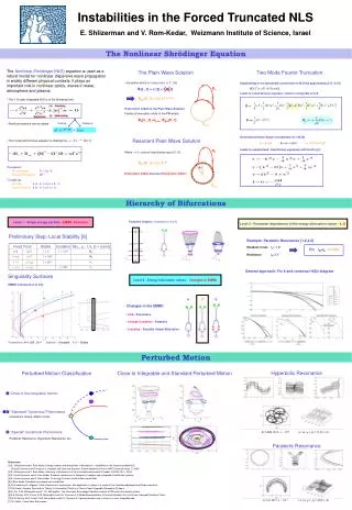
Instabilities in the Forced Truncated NLS Eli Shlizerman and Vered Rom-Kedar Weizmann Institute of Science 1. ES & RK, Characterization of Orbits in the Truncated NLS Model, ENOC-05 2. ES & RK, Hierarchy of bifurcations in the truncated and forced NLS model, CHAOS-05 3.ES & RK, Energy surfaces and Hierarchies of bifurcations - Instabilities in the forced truncated NLS, Cargese-03 SNOWBIRD, 2005
Near-integrable NLS (+) focusing • Conditions • Periodic Boundary u (x , t) = u (x + L , t) • Even Solutions u (x , t) = u (-x , t) • Parameters • Forcing Frequency Ω2 • Wavenumber k = 2π / L dispersion
Bh Homoclinic Orbits • For the unperturbed eq. • B(x , t) = c (t) + b (x,t) • Plain Wave Solution • Bpw(0 , t)= |c| e i(ωt+φ₀) • Homoclinic Orbit to a PW • Bh(x , t)t±∞Bpw(0 , t) Bpw [McLaughlin, Cai, Shatah]
Bh φ₀ Bpw Resonance – Circle of Fixed Points • When ω=0 – circle of fixed points occur • Bpw(0 , t)= |c| e i(φ₀) • Heteroclinic Orbits! [Haller, Kovacic]
Two Mode Model • Consider two mode Fourier truncation • B(x , t) = c (t) + b (t) cos (kx) • Substitute into the unperturbed eq.: [Bishop, McLaughlin, Forest, Overman]
General Action-Angle Coordinates for c≠0 • Consider the transformation: • c = |c| eiγb = (x + iy) eiγI = ½(|c|2+x2+y2) [Kovacic]
Then the 2 mode model is plausible for I < 2k2 Plain Wave Stability • Plain wave: B(0,t)= c(t) • Introduce x-dependence of small magnitude B (x , t) = c(t) + b(x,t) • Plug into the integrable equation and solve the linearized equation. From dispersion relation get instability for: 0 < k2 <|c|2
Hierarchy of Bifurcations • Level 1 • Single energy surface - EMBD, Fomenko • Level 2 • Energy bifurcation values - Changes in EMBD • Level 3 • Parameter dependence of the energy bifurcation values - k, Ω
Preliminary step - Local Stability B(x , t) = [|c| + (x+iy) coskx ] eiγ [Kovacic & Wiggins]
Level 1: Singularity Surfaces Construction of the EMBD - (Energy Momentum Bifurcation Diagram) [Litvak-Hinenzon & RK]
EMBD Parameters: k=1.025 , Ω=1 H4 H1 H3 H2 Dashed – Unstable Full – Stable
Fomenko Graphs and Energy Surfaces Example: H=const (line 5)
Level 2: Energy Bifurcation Values * 4 5* 6
I H Possible Energy Bifurcations • Branching surfaces – Parabolic Circles • Crossings – Global Bifurcation • Folds - Resonances
Finding Energy Bifurcations Resonance Parabolic GB
Parabolic Resonance: IR=IPk2=2Ω2 What happens when energy bifurcation values coincide? • Example: Parabolic Resonance for (x=0,y=0) • Resonance IR= Ω2 hrpw = -½ Ω4 • Parabolic Circle Ip= ½ k2 hppw = ½ k2(¼ k2-Ω2)
Level 3: Bifurcation Parameters Example of a diagram: • Fix k • Find Hrpw(Ω) • Find Hppw(Ω) • Find Hrpwm(Ω) • Plot H(Ω) diagram
Perturbed motion classification • Close to the integrable motion • “Standard” dyn. phenomena • Homoclinic Chaos, Elliptic Circles • Special dyn. phenomena • PR, ER, HR, GB-R
Homoclinic Chaos Model PDE k=1.025, Ω=1, ε ~ 10-4 i.c.(x, y, I, γ) = (0,0,1.5,π/2)
Hyperbolic Resonance Model PDE k=1.025, Ω2=1, ε ~ 10-4 i.c.(x, y, I, γ) = (0,0,1,π/2)
Parabolic Resonance Model PDE k=1.025, Ω2=k2/2, ε ~ 10-4 i.c.(x, y, I, γ) = (0,0,k2/2,π/2)
Classification y x Measure:σmax = std( |B0j| max)
Measure Dependence on ε p is the power of the order: O(εp)
Discussion • Solutions close to HR • Stability of solutions • Applying measure to PDE results