Download
1 / 35
350 likes | 478 Views
This course explores the theoretical underpinnings of longitudinal (single-bunch) instabilities in particle accelerators, focusing on observations from the CERN SPS in 2007. Participants will learn about single particle longitudinal motion, signal analysis, and the distribution of particles based on Hamiltonian dynamics. The course covers the impact of electromagnetic fields, the Liouville theorem, and stationary distributions on particle dynamics. Key concepts include phase space density, stationary effects, and implications for beam stability.

E N D
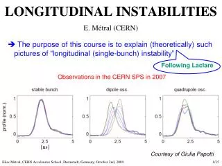
LONGITUDINAL INSTABILITIES E. Métral (CERN) • The purpose of this course is to explain (theoretically) such pictures of “longitudinal (single-bunch) instability” Following Laclare Observations in the CERN SPS in 2007 [ns] Courtesy of Giulia Papotti
SINGLE PARTICLE LONGITUDINAL MOTION (1/2) Time interval between the passage of the synchronous particle and the test particle, for a fixed observer at azimuthal position
SINGLE PARTICLE LONGITUDINAL MOTION (2/2) • Canonical conjugate variables • Linear matching condition • Effect of the (beam-induced) electromagnetic fields When following the particle along its trajectory
SINGLE PARTICLE LONGITUDINAL SIGNAL (1/3) • At time , the synchronous particle starts from and reaches the Pick-Up (PU) electrode (assuming infinite bandwidth) at times • The test particle is delayed by . It goes through the electrode at times • The current signal induced by the test particle is a series of impulses delivered on each passage Dirac function
SINGLE PARTICLE LONGITUDINAL SIGNAL (2/3) • Using the relations Bessel function of mth order Fourier transform
SINGLE PARTICLE LONGITUDINAL SIGNAL (3/3) • The single particle spectrum is a line spectrum at frequencies • Around every harmonic of the revolution frequency , there is an infinite number of synchrotron satellites m • The spectral amplitude of the mth satellite is given by • The spectrum is centered at the origin • Because the argument of the Bessel functions is proportional to , the width of the spectrum behaves like
DISTRIBUTION OF PARTICLES (1/2) • Signal induced (at the PU electrode) by the whole beam Number of particles per bunch • Canonically conjugated variables derive from a Hamiltonian by the canonical equations
DISTRIBUTION OF PARTICLES (2/2) • According to the Liouville’s theorem, the particles, in a non-dissipative system of forces, move like an incompressible fluid in phase space. The constancy of the phase space density is expressed by the equation • where the total differentiation indicates that one follows the particle while measuring the density of its immediate neighborhood. This equation, sometimes referred to as the Liouville’s theorem, states that the local particle density does not vary with time when following the motion in canonical variables • As seen by a stationary observer (like a PU electrode) which does not follow the particle => Vlasov equation
STATIONARY DISTRIBUTION (1/5) • In the case of a harmonic oscillator • Going to polar coordinates
STATIONARY DISTRIBUTION (2/5) • As r is a constant of motion • with A stationary distribution is any function of r, or equivalently any function of the Hamiltonian H
STATIONARY DISTRIBUTION (3/5) • In our case Amplitude of the spectrum • with
STATIONARY DISTRIBUTION (4/5) • Let’s assume a parabolic amplitude density • The line density is the projection of the distribution on the axis
STATIONARY DISTRIBUTION (5/5) • Using the relations Bunching factor • and
LONGITUDINAL IMPEDANCE All the properties of the electromagnetic response of a given machine to a passing particle is gathered into the impedance (complex function => in Ω)
EFFECT OF THE STATIONARY DISTRIBUTION (2/9) • Expanding the exponential in series (for small amplitudes) Synchronous phase shift Incoherent frequency shift (potential-well distortion) Nonlinear terms introducing some synchrotron frequency spread
EFFECT OF THE STATIONARY DISTRIBUTION (3/9) • Synchronous phase shift Test particle Synchronous particle • with
EFFECT OF THE STATIONARY DISTRIBUTION (4/9) Only for the small amplitudes. For the power loss of the whole bunch an averaging is needed! Can be used to probe the resistive part of the longitudinal impedance
EFFECT OF THE STATIONARY DISTRIBUTION (5/9) • Incoherent synchrotron frequency shift (potential-well distortion) • with • If the impedance is constant (in the frequency range of interest)
EFFECT OF THE STATIONARY DISTRIBUTION (6/9) • Using the relation For the parabolic amplitude density The change in the RF slope corresponds to the effective (total) voltage
EFFECT OF THE STATIONARY DISTRIBUTION (7/9) • Bunch lengthening / shortening (as a consequence of the shifts of the synchronous phase and incoherent frequency) The equilibrium momentum spread is imposed by synchrotron radiation • Electrons Neglecting the (usually small) synchronous phase shift • with
EFFECT OF THE STATIONARY DISTRIBUTION (8/9) The longitudinal emittanceis invariant • Protons Again, neglecting the (usually small) synchronous phase shift
EFFECT OF THE STATIONARY DISTRIBUTION (9/9) • General formula + for electrons and – for protons • Conclusion of the effect of the stationary distribution: New fixed point • Synchronous phase shift • Potential-well distortion
PERTURBATION DISTRIBUTION (1/2) Around the new fixed point • The form is suggested by the single-particle signal • Low-intensity Coherent synchrotron frequency shift to be determined Therefore, the spectral amplitude is maximum for satellite number m and null for the other satellites
PERTURBATION DISTRIBUTION (2/2) • with Amplitude of the perturbation spectrum • High-intensity
EFFECT OF THE PERTURBATION (1/10) • Vlasov equation with variables Linearized Vlasov equation
EFFECT OF THE PERTURBATION (2/10) • with Spectrum amplitude at frequency • with
EFFECT OF THE PERTURBATION (3/10) • Expanding the product (using previously given relations) Final form of the equation of coherent motion of a single bunch: Contribution from all the modes m
EFFECT OF THE PERTURBATION (4/10) • Coherent modes of oscillation at low intensity (i.e. considering only a single mode m) Multiplying both sides by and integrating over Twofold infinity of coherent modes
EFFECT OF THE PERTURBATION (5/10) • The procedure to obtain first order exact solutions, with realistic modes and a general interaction, thus consists of finding the eigenvalues and eigenvectors of the infinite complex matrix whose elements are • The result is an infinite number of modes ( ) of oscillation (as there are 2 degrees of freedom ) • To each mode, one can associate: • a coherent frequency shift (qth eigenvalue) • a coherent spectrum (qth eigenvector) • a perturbation distribution • For numerical reasons, the matrix needs to be truncated, and thus only a finite frequency domain is explored The imaginary part tells us if this mode is stable or not
EFFECT OF THE PERTURBATION (6/10) • The longitudinal signal at the PU electrode is given by • For the case of the parabolic amplitude distribution
EFFECT OF THE PERTURBATION (7/10) • Low order eigenvalues and eigenvectors of the matrix can be found quickly by computation, using the relations • The case of a constant inductive impedance is solved in the next slides, and the signal at the PU shown for several superimposed turns
EFFECT OF THE PERTURBATION (8/10) Signal observed at the PU electrode DIPOLE mode QUADRUPOLE mode
EFFECT OF THE PERTURBATION (9/10) • The spectrum of mode mq • is peaked at • and extends • There are q nodes on these “standing-wave” patterns SEXTUPOLE mode
EFFECT OF THE PERTURBATION (10/10) Observations in the CERN SPS in 2007 (Laclare’s) theory