Download

1 / 32
330 likes | 459 Views
Site Productivity and Land Classification. Lecture 13: Forest Ecology 550. Objectives. Discuss indirect ways to measure site productivity Briefly discuss land classification Introduce ecosystem process models

E N D
Site Productivity and Land Classification Lecture 13: Forest Ecology 550
Objectives • Discuss indirect ways to measure site productivity • Briefly discuss land classification • Introduce ecosystem process models • What role can remote sensing play in estimating forest species composition, structure, and function.
Site Productivity • Definition • Sites potential to produce one or more natural resources • Sustainable • Manage for multiple resources
Site Productivity: indirect measurement approaches • 1) Site index: Forest measurement to measure site quality • Based on height of the dominant and co-dominant trees based on some standard age • Age depends on location and stand type • Typically 50 years but..
Pros Easy and inexpensive Height growth is less sensitive than basal area growth to stocking density. Cons very site dependent (soils, topography, aspect) Differs among species Requires trees growing on the site Cannot capture dynamic nature of tree growth and global change Site index curves: Pros/cons
Site Productivity: indirect measurement approaches • 2) Overstory tree species • Each species occupies its own niche
Site Productivity: indirect measurement approaches • 2) Overstory tree species • Each species occupies its own niche • Advantages • Allows you to make quick assumptions about a given area • Disadvantages • Challenging for species that are able to exist in a wide range of climates
Site Productivity: Indirect measurement approaches • 3) understory species • Definition: use of understory species to make classifications of site • Advantages: • More sensitive to micro-climate differences • Indicator species • Disadvantages • What about disturbance
Site Productivity: Indirect measurement approaches • 3) understory species • Other examples: • Ephemerals often have a narrow ecological niche
Site Productivity: Indirect measurement approaches • 4) Ecological Site Classification • Primary means is through Habitat Typing • Identified by distinct understory plant assemblages • natural vegetation to identify ecologically equivalent landscape units • growth • natural resource use potential
Soil usually sand to loamy sand. At least two species present:low sweet blueberry, wintergreen, sweet fern, pipsissewa, cow wheat, witch hazel, maple-leaf viburnum, pointed leaf tick treefoil witch hazel, maple-leaf viburnum, pointed leaf tick treefoil Species on right rare or absent blueberry, wintergreen Species on right rare or absent At least 2 present honeysuckle, twisted stalk, partridgeberry, yellow beadlilly, shield fern, ironwood Sum of the coverage > 2x’s the sum of species In right box trailing arbutus, bear berry, reindeer moss hazelnut, false Soloman’s seal, barren strawberry AQVib PMV QAE AQV
Examples of WI Habitat Types Maianthemum Coptis Sweet anise/osmorhiza
Habitat Types: Comparisons in WI • Litterfall C and N generally increase from low quality to high quality habitat type
Habitat Types • Advantages • Fairly detailed • Qualitative formulae • Disadvantages • May take some time to identify the factors in the stand
Site Productivity: Indirect Measurement Approaches • 5) Environmental Relationships/factors • Simple relationships between one of more variable and tree growth. • from E.C. Steinbrenner. 1981. Forest soil productivity relationships. In Forest Soils of the Douglas-fir Region).
Environmental relationships/factors cont.. • from E.C. Steinbrenner. 1981. Forest soil productivity relationships. • In Forest Soils of the Douglas-fir Region).
Environmental relationships/factors cont.. ANPP Leaf biomass
Site Productivity: Indirect Measurement Approaches • 6) Ecosystem Process Models • based on biophysical and ecological principles • every physiological process model has some level of empiricism
General Outline for the conceptual framework of biome-BGC PPT evaporation LAI transpiration LAI Soil water photosynthesis Soil water outflow respiration
Site Productivity: Indirect Measurement Approaches • 7) Remote Sensing • Common Vegetation indices derived from radiation reflectance measured using satellites • Simple ratio = (near infra-red(NIR)/red (R) wavelength) • Normalized Difference Vegetation Index • (NDVI)= (NIR - R)/(NIR + R)
Site Productivity: Indirect Measurement Approaches • 7) Remote Sensing • Normalized Difference Vegetation Index • (NDVI)= (NIR - R)/(NIR + R)
ETM+ predictions of Aug. LAI Corn LAI=4.00+0.45*CCIca R2=0.63 Soy LAI=3.44+0.49*CCIsa R2=0.27 ETM+ predictions of July LAI Corn LAI=4.41+0.63*CCIcj R2=0.61 Soy LAI=1.54+0.49*CCIsj R2=0.58 Predicted versus Measured LAI
RMSE=9.09 Slope=0.98 Intercept=1.46 R=0.84 RMSE=1.19 Slope=1.00 Intercept=0.10 R=0.74 1:1 1:1 Canonical indices ETM+ March, June Canonical indices ETM+ March, June
Modis GPP project • GPP (gC m-2 d-1) = PAR * fAPAR * g • Where: • PAR = from climate model • fAPAR = from MODIS reflectances • g ( gC MJ-1) = GPP / APAR • MODIS g from lookup table • Spatial Resolution is 1 km • Temporal Res. is 8-day mean
Remote Sensing Disturbance 98 1995 1989 81 50 km - Disturbances are an important component of any forest ecosystem - Disturbances have no effect on the C budget if the system is in steady state Fire frequency and extent has increased 270% in recent decades In Saskatchewan and Manitoba
Hudson Bay 2003 NDVI 3-date Composite max leaf area Fire date leaf expansion 2003 fire snowmelt Fire scar profiles taken from 2003 NDVI seasonal data. Selected burn areas shown in image on the right. 2002 MODIS Image Manitoba-Saskatchewan