Download
1 / 27
270 likes | 396 Views
This article delves into advanced genetic algorithms (GAs) capable of solving complex problems efficiently and reliably. It discusses various types of GAs such as Messy GAs, Learning Linkage GAs, and Compact GAs, highlighting their unique properties and applications. Key techniques like probabilistic model building, extended thresholding, and gene strength adjustment mechanisms are examined, illustrating how these methods enhance performance on high-dimensional, multimodal problems. The potential for evolutionary inspirations in algorithm design is also explored.

E N D
Competent GAs • Can solve • hard problems (multimodal, deceptive, high degree of subsolution interaction, noise, ...), • quickly, • accurately, • reliably. • Messy GAs – mGA, fmGA, gemGA • Learning linkage GAs – LLGA • Compact GAs – cGA, ECGA • Bayesian optimization algorithm - BOA
Messy GAs • Inspirationfrom the nature – evolution starts from the simplest forms of life • Tagged alleles: • Variable-length strings: (name1, allele1) … (nameN, alleleN) ((4,0) (1,1) (2,0) (4,1) (4,1) (5,1)) • Over-specification – multiple gene instances • Underspecification – missing gene instances • Messy operators: cut & splice • Initialization • Enumerative initialization of the population with all sub-strings of a certain length k<<l (lk)2k O(lk) computations • Guaranteed that all BBs of certain size are present in the population
Fast messy genetic algorithms - fmGAs • Probabilistically complete enumeration • Population of strings of length l’ close to l is generated • Assumption: each string contains many different BBs of length k<<l • Building block filtering – extracts highly-fit and effectively linked BBs • Repeated (1) selection and (2) gene deletion • Only O(l) computations to converge • Extended thresholding – tournaments are held only between strings that have a threshold number of genes in common • fmGA vs mGA: 150-bit long problem, 305-bit deceptive func. • 1.9105 vs. 5.9108 evaluations
Gene expression messy GA - gemGA • Messy ??? • No variable-length strings • No under- or over-specification • No left-to-right expression • Messy use of heterogeneous phases of processing • Linkage learning phase - first identifies linkage groups • Mixing phase – selection + recombination • exchanges good allele combinations within those groups to find optimal solution
gemGA: The idea • Linkage learning phase • Transcription I (antimutation) • Each string undergoes l one-bit perturbations • Improvements are ignored ?!? (bit does not belong to optimal BB) • Changes that degrade the structure are marked as possible linkage groups candidates Ex.: two 3-bit deceptive BBs 111 101 marked not marked (degrades) (improves) • Transcription II • Identifies the exact relations among the genes by checking nonlinearities IF f(X’i) + f(X’j) != f(X’ij) THEN link(i,j)
Probabilistic Model-Building GAs • Initialize population at random • Select promising solutions • Build probabilistic model of selected solutions • Sample built model to generate new solutions • Incorporate new solutions into original population • Go to 2 (if not finished)
Extended compact GA - ECGA • Marginal product model (MPM) • Groups of bits (partitions) treated as chunks • Partitions represent subproblem • Onemax: [1] [2] [3] [4] [5] [6] [7] [8] [9] [10] • Traps: [1 2 3 4 5] [6 7 8 9 10]
Learning structure in ECGA • Two components • Scoring metrics: minimal description length (MDL) • Number of bits for storing probabilities: Cm = log2Ni 2Si • Number of bits storing population using model: Cp = NiE(Mi) • Minimize C = Cm + Cp • Search procedure: a greedy algorithm • Start with one-bit groups • Merge two groups for most improvement • No more improvement possible finish.
BB: ECGA model
GA s reálně kódovanou binární rep. (GARB) • Pseudo-binární rep.- bity kódovány reálným číslem r 0.0, 1.0 • interpretace(r) =1, pro r> 0.5 = 0, pro r < 0.5 redundance kódu • Příklad: ch1 = [0.92 0.07 0.23 0.62] ch2 = [0.65 0.19 0.41 0.86] interpretace(ch1) = interpretace(ch2) = [1 0 0 1] • Síla genů – vyjadřuje míru stability genů • Čím blíže k 0.5 tím je gen slabší (nestabilnější) • „Jedničkové geny“: 0.92 > 0.86 > 0.65 > 0.62 • „Nulové geny“: 0.07 > 0.19 > 0.23 > 0.41
Gene-strength adjustment mechanism • Geny chromozomů vzniklých při křížení jsou upraveny • v závislosti na jejich interpretaci • a relativní frequenci jedniček (nul) na dané pozici v populaci P[] př.: P[0.82 0.17 0.35 0.68] v populaci je na 1. pozici 82% jedniček, na 2. pozici 17% jedniček, na 3. pozici 35% jedniček, na 4. pozici 68% jedniček. • Geny, které v populaci převládají jsou oslabovány; ostatní jsou posilovány.
Posilování a oslabování genů • Oslabování gen’ =gen+c*(1.0-P[i]), když (gen<0.5) a (P[i]<0.5) (gen má hodnotu nula a v populaci na i-té pozici převažují nuly) a gen’ = gen – c*P[i], když (gen>0.5) a (P[i]>0.5) • Posilování gen’ = gen – c*(P[i]), když (gen<0.5) a (P[i]>0.5) (gen má hodnotu nula a v populaci na i-té pozici převažují jedničky) a gen’ = gen + c*(1.0-P[i]), když (gen>0.5) a (P[i]<0.5) • Konstanta c určuje rychlost adaptace genů: c (0.0,0.2
Stabilizace slibných jedinců • Potomci, kteří jsou lepší než jejich rodiče by měli být stabilnější než ostatní vygenerovaná nekvalitní řešení • Chromozomy slibných jedinců jsou vygenerovány se silnými geny ch = (0.71, 0.45, 0.18, 0.57) ch’= (0.97,0.03, 0.02, 0.99) • Geny slibných jedinců přežijí více generací aniž by byly zmeněny v důsledku oslabování
GARB: Generační model • inicializace generuj(OldPop) P[i]=0,5 pro i=1...lchrom • repeat N=0 repeat rod1, rod2 vyber(OldPop) pot1, pot2 zkřiž(rod1, rod2) stabilizuj(pot1, pot2) NewPop vlož(pot1, pot2) N = N + 2 until(N <PopSize) uprav(P[], NewPop) OldPop NewPop until(neplatí ukončovací podmínka)
GARB: Steady-state model • inicializace generuj(OldPop) P[i]=0,5 pro i=1...lchrom • repeat rod1, rod2 vyber(OldPop) pot1, pot2 zkřiž(rod1, rod2) oslab(rod1, rod2) stabilizuj(pot1, pot2) najdi(odpadlík) OldPop[odpadlík] vlož(pot2) uprav(P[], OldPop) statistika until(neplatí ukončovací podmínka)
Testovací úlohy - statické • F101(x, y) • Deceptive function • Hierarchická funkce
Testovací úlohy - dynamické • Ošmerův dynamický problém g(x,t) = 1-exp(-200(x-c(t))2) c(t) = 0,04(t/20) • Minimum g(x,t)=0.0se mění každých 20 generací • Oscillating Knapsack Problem 14 objektů, wi=2i, i=0,...,13 f(x)=1/(1+target-wixi) • Target osciluje mezi hodnotami 12643 a 2837, které se v binárním vyjádření liší o 9 bitů
DF H-IFF F101 Výsledky na statických problémech
Výsledky na dynamických problémech Oscillating knapsack problem
MTE – Mean Tracking Error[%] – střední odchylka nejlepšího jedince v populaci a optimálního řešení počítaná přes všechny gen. Bezprostředně po změně opt. Celkově Algoritmus MTEStDevMTEStDev GARBc = 0:12512.822.41.03.9 SGA binaryN/AN/A57.343.61 SGA GrayN/AN/A47.6642.94 CBM-BN/AN/A19.3933.13 Výsledky na dynamických problémech • Ošmerův dynamický problém