Hartree – Fock Benchmark

Hartree – Fock Benchmark JOHN FEO Center for Adaptive Supercomputing Software

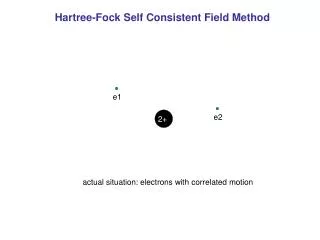
Self-Consistent Field Method • Obtain variational solutions to the electronic Schrödinger Equation Energy Wavefront • By expressing the system’s one electron orbitals as the dot product of the system’s eigenvectors and some set of Gaussian basis functions eigenvector Gaussian basis function

… reduces to • The solution to the electronic Schrödinger Equation reduces to the self-consistent eigenvalue problem Fock matrix Eigenvectors Density matrix Overlap matrix Eigenvalues One-electron forces Two-electron Coulomb forces Two-electron Exchange forces

Logical flow Initial Density Matrix Construct Fock Matrixa) One electronb) Two electron Initial Orbital Matrix Compute Orbitals Schwarz Matrix no convergence Compute Density Matrix Damp Density Matrix convergence Output

Modules denges Construct Fock Matrixa) oneelb) twoel makeob diagon makesz no convergence a) dampb) dendif makden convergence Output

Matrix flow Compute Fock Matrix g_schwartz h g_schwartz g g_fock diagon oneel twoel g_fock eigv g_dens g_orbs g_work makden Damp Density Matrix dendif - constant - current iteration Output - previous iteration

Memory footprint • Ten 2-D arrays of size nbfn x nbfn • Two 1-D arrays of size nbfn • h is size (nbfn)2 • gis size (nbfn)4 • Direct method – compute g each time • Conventional method – compute g once and store nbfn = number of basis functions = 15 * number of atoms

Typical loop structures oneel for (i = 0; i < nbfn; i++) {for (j = 0; j < nbfn; j++) {g_fock[i][j] = (g_schwarz[i][j] > tol) ? h(i,j) : 0.0;} } makden for (i = 0; i < nbfn; i++) {for (j = 0; j < nbfn; j++) { double p = 0.0; for (k = 0; k < nocc; k++) p += g_orbs[i][k] * g_orbs[j][k];g_work[i][j] = 2.0 * p;} } nocc = 2 * number of atoms dendif for (i = 0; i < nbfn; i++) {for (j = 0; j < nbfn; j++) { double xdiff = fabs(g_dens[i][j] – g_work[i][j]); if (xdiff > denmax) denmax = xdiff;} }

The BIG loop twoel for (l = 0; l < nbfn; l++) {for (k = 0; k < nbfn; k++) {for (j = 0; j < nbfn; j++) {for (i = 0; i < nbfn; i++) { if (g_schwarz[i][j] * schwmax ) < tol2e) {icut1 ++; continue;} if (g_schwarz[i][j] * g_schwarz[k][l]) < tol2e) {icut2 ++; continue;} icut3 ++; double gg = g(i, j, k, l);g_fock[i][j] += ( gg + g_dens[k][l]);g_fock[i][k] -= (0.5 * gg * g_dens[j][l]);} } } }

Optimizations • Tiling to improve locality and data reuse • e.g. - twoel • Module collapse to increase thread size and reduce memory operations • e.g. - makden and dendif • Inline g and hoist loop invariant subexpressions • Exploit 8-way symmetry of g --- precompute and save • Conventional method (compute h and g once and store) • Probably enough memory • Probably not enough latency tolerance or power

Hartree – Fock Benchmark