Download
1 / 33
330 likes | 608 Views
TSV-Aware Analytical Placement for 3D IC Designs. Meng-Kai Hsu, Yao-Wen Chang, and Valerity Balabanov GIEE and EE department of NTU DAC 2011. Outline. Introduction Previous works and Contributions Problem formulation and analytical placement TSV-aware 3D analytical global placement

E N D
TSV-Aware Analytical Placement for 3D IC Designs Meng-Kai Hsu, Yao-Wen Chang, and Valerity Balabanov GIEE and EE department of NTU DAC 2011
Outline • Introduction • Previous works and Contributions • Problem formulation and analytical placement • TSV-aware 3D analytical global placement • TSV insertion and TSV-aware legalization • Experimental results and Conclusions
Introduction • 3D IC technology can effectively reduce global interconnect length and increase circuit performance. • In a generic 3D IC structure, each die is stacked on top of another and communicated by Through-Silicon Vias (TSVs).
Introduction (cont.) • TSV pitches are very large compared to the sizes of regular metal wires under current technology. • Moreover, TSVs are usually placed at the white space. • Routing resource, chip area, yield, etc. are affected.
Previous works • [9] folding/stacking with layer re-assignment. • [11] use partitioning-based approach. • [7] is multi-level analytical placement and cell could move along z-direction. • [15] partition cell first, then do placement for each layer.
Contributions • New 3D placement algorithm consists of three stages that takes sizes and positions of TSVs into account. • Weighted-average wirelength model with smaller estimation errors than Log-sum-exp (LSE) model. • Density cube to model the density.
Contributions (cont.) • Not only handles the TSV count but also handles the size of TSVs. • A TSV insertion algorithm based on the overlapping whitespace area between neighboring layers is proposed to determine the location of each TSV. • Routing can be easily accomplished. Moreover, the proposed algorithm achieves best comparing with [7,15].
Problem formulation • Given a placement region and the number of device layers k, we intend to determine the optimal positions of movable blocks so that the total wirelength and the number of required TSVs are minimized while satisfying the non-overlapping constraints among blocks and TSVs. • Inputs • as the set of n blocks. • as the set of m nets. • Placement region definitions with k device layers. • Density constraints, TSV size. • Outputs • The location of each block and TSVs (layer and coordinates) without constraint violation. The netlist should be updated.
Traditional placement flow • Global placement: Find the best position and layer for each block to minimize the target cost. • Legalization: Remove overlaps. • Detail placement: Refines the placement solution.
Analytical placement • Optimize the target of placement by mathematical way. • Linear programming (LP), Quadratic programming (QP), etc. • Key: How to model and how to solve.
3D analytical global placement • The 3D analytical global placement problem can be formulated as a constrained optimization problem as follows:
Wirelength and TSV model • The wirelength W(x, y) is defined as the total half-perimeter wirelength (HPWL). • The number of TSVs used for each net could be approximated by the number of layers it spans.
Wirelength and TSV model (cont.) • The above equations is not differentiable. • Need differentiable one to approximate. • Log-sum-exp (LSE) model • The LSE wirelength is close to the HPWL when γ approaches to zero. • In fact, γ cannot be too small or else overflow occurs => error is inevitable.
Proposed weighted-average (WA) wirelength model • Weighted-average • In order to approximate maximum, the following function is used. • Hence, the WA model will be:
Density cube model • The density of a cube b of layer k can be defined as: • Px, Py, and Pz are the overlap computing functions along three dimensions.
White space reservation for TSVs • Assume that the communication between neighboring layers of a net is through one TSV. • Distribute required spaces for TSVs into density cubes inside the net-box evenly. • Net-box: the range spanned by a net.
Transform to unconstrained problem • Solve a sequence of unconstrained problem with increasing λ.
TSV insertion and TSV-aware legalization • Three-step scheme • Layer-by-layer standard cell legalization • TSV insertion • TSV-aware legalization • Layer-by-layer standard cell legalization • Minimum cell displacement without considering TSVs. • Just like traditional legalization.
TSV insertion and TSV-aware legalization (cont.) • TSV insertion • Decompose each net to 2-pin nets by MST. • Start from the 2-pin net with the smallest net-box to the largest one. • Divide the region enclosed by net-box into bins, and insert TSV into the overlapping white space bin with minimized overlap between cells and TSVs. • If there is not enough white space in the net-box, the searched region is doubled, and the search process continues.
Decompose each net to 2-pin nets by MST • Project cells to a single layer, then compute edge cost by β*L(e)+δ*Z(e).
TSV insertion and TSV-aware legalization (cont.) • TSV-aware legalization • Apply step1 and set TSVs as fixed blocks.
Experimental results • Environment • PC workstation • 8x Xeon 2.5 GHz CPUs • 26 GB memory • Implemented using C++ • Integrated into NTUplace3 • α ,β, and γ are set to 10, 0.4, and 0.6 respectively.
3D analytical placement comparisons • 4-layer 3D IC, area of each layer is (original area)/4 and then enlarge to get 10% white space.
Conclusions • Proposes a new TSV-aware placement algorithm for 3D design. • Weighted-average wirelength model. • White space reservation for TSV insertion. • Routing could easily be done by 2D routers, and the algorithm achieves the best result among [7,15].