Probabilistic Weather Forecasting Using Bayesian Model Averaging

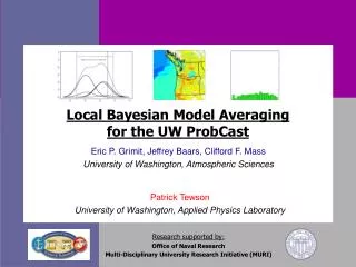
Probabilistic Weather Forecasting Using Bayesian Model Averaging J. McLean Sloughter Adviser: Tilmann Gneiting GSR: Susan Joslyn Committee members: Adrian Raftery & Cliff Mass 8 May, 2009 This work was supported by MURI, JEFS, & NSF grants

Background • Motivation • Ensemble forecasting • Bayesian model averaging • Dissertation outline • BMA for vector wind • Data • Decomposing the problem • Bias-correction • Error distributions • Model • Results • Future directions • References • Acknowledgements

Why probabilistic forecasting? • Situations where certain ranges or thresholds are of interest • Situations where knowing not just the most likely outcome, but possible extremes are important • Situations involving a cost / loss analysis, where probabilities of different outcomes need to be known • Examples: • Wind energy • Military • Sailing • Airports • Winter road maintenance

Ensemble Forecasting 48-hour forecasts for maximum wind speeds on 7 August 2003

Ensemble Forecasting • Single forecast model is run multiple times with different initial conditions • Forecasts created on a 12-km grid, and bilinearly interpolated to locations of interest • Ensemble mean tends to outperform individual members • Spread-skill relationship: spread of forecasts tends to be correlated with magnitude of error

Ensemble Forecasting • Would like the ensemble to look like draws from the same distribution as the observed values • Ensemble only captures one source of variability – uncertainty in initial conditions • Ensemble distribution is underdispersed relative to observed values • Ensemble members agree with one another more than they agree with observations

Bayesian model averaging (BMA) • Weighted average of multiple component models • One component per ensemble member • Each component a distribution of observed value conditioned on an ensemble member forecast • Model fit based on training data – past sets of forecasts / observations • Use a sliding window of training data • Weights determined by how well each member fits the training data

Bayesian model averaging where is the deterministic forecast from member k, is the weight associated with member k, and is the estimated density function for y given member k

Dissertation Outline • Precipitation forecasting • Sloughter et al., 2007, MWR • Extends BMA to a specific case of skewed and non-continuous distributions • Wind speed forecasting • Sloughter et al., 2009, JASA • Extends methods of Sloughter et al. (2007) to other forms of skewed and non-continuous distributions • Examines robustness of BMA to details of model selection • Vector wind forecasting • This talk • Extends BMA to multivariate distributions

BMA for vector wind • Methods exist for using Bayesian Model Averaging to create probabilistic forecasts for weather quantities that can be expressed as a mixture of normals (Raftery et al., 2005), such as temperature and pressure. • Expanded to be applied to non-continuous and skewed quantities such as precipitation and wind speed in Sloughter et al. 2007, Sloughter et al. 2009. • A method is needed for modeling multivariate quantites such as wind vectors.

Knot • A knot is a measure of speed used in nautical, meteorological, and aviation settings • 1.852 kilometers per hour • 1.151 miles per hour • 0.514 meters per second • Sailors would throw out the chip log (a board designed to stay stationary in water) tied to a rope with knots spaced 7 fathoms (42 feet) apart • They would then count how many knots were fed out in 30 seconds

Knot • 4-6 knots is a light breeze – leaves move, breeze can be felt on one’s face • 11-16 knots is a moderate breeze – dust and paper will be blown about, whitecaps will form on the water • 20-21 knots is generally the threshold for issuing a small craft advisory • 34-40 knots is a gale – small branches break from trees, walking becomes difficult

Data • This work uses wind data from the Pacific Northwest for the full year 2003, plus November and December 2002 (results for 2003 data, 2002 used only for training) • “Instantaneous” vector wind measurements • Measured in knots • Each forecast consists of 8 ensemble members • Data were available for 343 days, missing for 83 days • A total of 38091 observations, averaging 111 observations per day • All work that follows is based on 30-day training periods, with 2-day-ahead forecasting

Data • Data from Surface Airway Observation stations • Airports in BC, Washington, Oregon, Idaho, and California

Decomposing the problem • Wind has two dimensions, east/west direction and north/south direction • BMA uses a mixture distribution with one component per ensemble member • Consider each mixture component a bivariate distribution parameterized in terms of a mean vector and a covariance matrix • Assume that the mean of the distribution is some function of the forecast vector, and that the covariance matrix does not depend upon the forecast (exploratory plots support these assumptions)

Decomposing the problem • h(fk)is the mean (a bias-corrected forecast) • BV(0, Q) is the distribution of the forecast error • Model the distribution of the errors rather than the observed values • Has the advantage of having constant parameters across forecast values • Can then be decomposed into two separate problems: • bias-correcting the forecast • modeling the error distribution

Bias-correction • For simplicity, consider affine bias corrections • Two potential forms of bivariate bias correction • Additive bias-correction • Full affine bias-correction • Where Y is the observed wind vector, fk is the kth vector forecast, ak is an additive bias vector, and Bk is a transformation matrix

Bias-correction Bivariate root mean squared error (in knots) for one ensemble member • Out-of-sample results using 30-day training period • Similar results hold for other ensemble members • Affine bias-correction shows a marked improvement

Error distributions • Now deal with the error field (observations minus bias-corrected forecasts) • Exploratory work suggests that the distributions are ellipsoidal, but have heavier tails than normal distributions • Transform the error vector (rkcosqk, rksinqk)T by raising the magnitude of the vector to the 4/5 power while preserving the angle • Model this as a bivariate normal distribution

Model • Thus, our final model is: • Where the gk are the distributions on y implied by the distributions of the transformed error vectors • Model parameters are estimated globally using all observation locations

Model • Bias-correction fit via linear regression (separate bias correction for each mixture component) • Weights and covariance matrix estimated via maximum likelihood using the EM algorithm • Use latent variables zkst which are indicators that forecast k was the best forecast at station s at time t

Model • E step: • M step:

Model • M step (continued)

Results • We simulate a large number of forecasts from our distribution • Can evaluate the forecast of either the wind vector or derived quantities (marginal speed or direction) from the empirical distribution of our forecasts • Essentially creating a new, larger ensemble of forecasts that should be better-calibrated than the original ensemble

Example • To illustrate what the BMA distribution is doing, consider the case of forecasting at Omak, Washington on February 4th, 2003

Results • Our goal is to maximize sharpness subject to calibration (the Gneiting principle) • By calibration, we mean that we want our probability distribution function to be correct – if we forecast an event as happening with probability .9, we want it to happen 90% of the time • By sharpness, we mean that we want predictive intervals to be as narrow as possible

Results • For univariate quantities, the verification rank histogram is a tool that can be used to assess the calibration of an ensemble forecast • Find the rank of each forecast relative to the ensemble members • If the ensemble is properly calibrated, the observation and forecasts should be interchangeable • If so, each potential rank of the forecast should have equal probability • Thus, a histogram of the ranks should look flat

Results • For multivariate quantities, there is an analogous multivariate rank histogram (MVRH), again based on the assumption of exchangeability • Define if and only if in every dimension • For each member of the combined set of the observation and the forecasts, find the pre-rank • The multivariate rank is the rank of the observation pre-rank, with any ties resolved at random • If we have a set of 8 forecasts and 1 observation, there are 9 possible rankings of the observation relative to the forecasts

Results • MVRH for the raw ensemble (left) and BMA forecast distribution (right) • Raw ensemble is under-dispersed • BMA forecast distribution is much better-calibrated

Results • The energy score (ES) is a scoring rule for multivariate probabilistic forecasts that takes into account both calibration and sharpness • In the univariate case, it reduces to the continuous ranked probability score (CRPS) • P is the predictive distribution, x the observed wind vector, X and X’ independent random variables with distribution P

Results • There may still be interest in a point forecast as well • We can use the spatial median as a point forecast • We can assess the quality of a multivariate point forecast using the multivariate mean absolute error (MMAE)

Results • BMA outperforms climatology and the raw ensemble both in terms of the probabilistic forecast and the deterministic forecast

Results – marginal speed and direction • Again consider verification rank histograms to assess calibration • Both speed (top) and direction (bottom) are much improved by BMA

Results – marginal speed and direction • CRPS is the scalar equivalent of the energy score • DCRPS is the angular equivalent • Scalar point forecasts can be assessed by the MAE, and angular point forecasts by the mean directional error (MDE) • Can also look at coverage and width of 77.8% prediction intervals for scalar forecasts – coverage assesses calibration, width assesses sharpness

Results – marginal speed and direction • Wind speed: • Wind direction:

Results – marginal speed and direction • We can see that for both speed and direction, BMA improves the quality of both the probabilistic and deterministic forecasts • BMA produces marginal distributions that are better-calibrated than the raw ensemble and sharper than climatology

Future Directions • Develop a BMA method to explicitly model marginal instantaneous wind speed and compare to the performance of the forecasts from this model (current BMA for marginal wind speed is for maximum wind speeds, not instantaneous) • Incorporate spatial information, either through explicitly modeling some spatial structure to our parameters or by estimating parameters locally rather than globally • Investigate using an exponential forgetting for training data rather than a sliding window, which could allow for faster computation through the use of updating formulae for parameter estimates • Extend multivariate methods to jointly forecast multiple weather quantities simultaneously

References • Raftery, A.E., Gneiting, T., Balabdaoui, F. and Polakowski, M. (2005). Using Bayesian Model Averaging to calibrate forecast ensembles. Monthly Weather Review, 133, 1155-1174. • Sloughter, J. M., Raftery, A. E., Gneiting, T. and Fraley, C. (2007). Probabilistic quantitative precipitation forecasting using Bayesian model averaging. Monthly Weather Review, 135, 3209-3220. • Sloughter, J. M., Gneiting, T., and Raftery, A.E. (2009). Probabilistic wind speed forecasting using ensembles and Bayesian model averaging. Journal of the American Statistical Association, accepted. • Mass, C., Joslyn, S., Pyle, P., Tewson, P., Gneiting, T., Raftery, A., Baars, J., Sloughter, J. M., Jones, D., and Fraley, C. (2009). PROBCAST: A web-based portal to mesoscale probabilistic forecasts. Bulletin of the American Meteorological Society, in press. • http://probcast.com

Acknowledgements • Committee: • Tilmann Gneiting - adviser • Adrian Raftery, Cliff Mass - committee members • Susan Joslyn - GSR • Statistics folks: • Veronica Berrocal, Chris Fraley, Thordis Thorarinsdottir, Will Kleiber, Larissa Stanberry, Matt Johnson, Robert Yuen, Michael Polakowski, Nicholas Johnson • Atmospheric Sciences folks: • Jeff Baars, Eric Grimit, Jeff Thomason, Tony Eckel • APL folks: • Patrick Tewson, John Pyle, David Jones, Janet Olsonbaker, Scott Sandgathe • Psychology folks: • Limor Nadav-Greenberg, Buzz Hunt, Queena Chen, Jared Le Clerc, Rebecca Nichols, Sonia Savelli

Probabilistic Weather Forecasting Using Bayesian Model Averaging