Convolution, Impulse Response, Filters

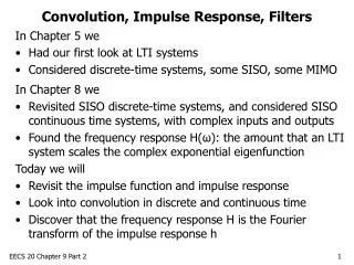
1. Convolution, Impulse Response, Filters In Chapter 5 we • Had our first look at LTI systems • Considered discrete-time systems, some SISO, some MIMO In Chapter 8 we • Revisited SISO discrete-time systems, and considered SISO continuous time systems, with complex inputs and outputs • Found the frequency response H(ω): the amount that an LTI system scales the complex exponential eigenfunction Today we will • Revisit the impulse function and impulse response • Look into convolution in discrete and continuous time • Discover that the frequency response H is the Fourier transform of the impulse response h EECS 20 Chapter 9 Part 2

2. Convolution In Chapter 5, we defined a mathematical operation on discrete-time signals called convolution, represented by  . Given two discrete-time signals x1 , x2  [Integers → Reals], • n  Integers, We can also define convolutions for continuous-time signals. Given two continuous-time signals x1 , x2  [Reals → Reals], • t  Reals, EECS 20 Chapter 9 Part 2

3. Properties of Convolution Convolution is commutative: x1  x2 = x2  x1 . Convolution is associative: (x1  x2)  x3 = x1  (x2  x3) . Convolution also has the following properties: for scalars a, These stem from the fact that integration and summation have additivity and homogeneity properties. EECS 20 Chapter 9 Part 2

4. Defining LTI Systems Using Convolution In addition to using (A, B, C, D) or writing out a difference or differential equation, we may define an LTI system using convolution. Take any discrete-time function g  [Integers → Reals]. The convolution defines an LTI system S. The output for any input is obtained through convolution. The properties of convolution ensure that S is LTI. When we define a system this way, we call the defining function g the convolution kernel. This method may be used to define continuous-time systems too. EECS 20 Chapter 9 Part 2

5. Example Consider the system defined by the kernel • t  Reals, g(t) = The output of this system for any input x is The output is the average value of x over the last 3 time units. { 1/3 if t  [0, 3] 0 otherwise EECS 20 Chapter 9 Part 2

6. Impulse Response as Kernel Recall that we have already defined an LTI system using a kernel. In Chapter 5, we showed that the output for a discrete-time SISO LTI system can be given by the convolution of the input and the impulse response h: Remember that the impulse response is the particular system output obtained when the input is the Kronecker delta function • n  Integers, (n) = { • if n = 0 • 0 if n ≠ 0 EECS 20 Chapter 9 Part 2

7. Dirac Delta Function We define the impulse response h for a continuous-time system as the output for a particular input called the Dirac delta function. The Dirac delta function is not really a function. We define the Dirac delta function δ: Reals→Reals to have the following properties: t  Reals \ {0}, δ(t) = 0 ε  Reals with ε>0, EECS 20 Chapter 9 Part 2

8. Dirac Delta Function So the Dirac delta function δ(t) has infinite value at t=0, and is zero everywhere else. Yet, the area under the function is equal to 1. If we scale the function by a, the function aδ(t) will still be zero for all nonzero t and infinite at t = 0. But, the area under the function will now equal a. We draw the Dirac delta function as an arrow pointing up at t=0 indicating its infinite value there. The height of the arrow represents the weight, the area under the function. δ(t) 1 t EECS 20 Chapter 9 Part 2

9. Sifting Property Both the Kronecker and Dirac delta functions have the following property: When a signal is convolved with a delta function, it remains unchanged. This is called the sifting property. For the discrete-time case, we see that the delta function is zero for all k except k = n. So there is only one term in the sum, x(n)δ(n-n) = x(n). For the continuous time case, δ(t-) will be nonzero only for =t. So it doesn’t matter what δ(t-) multiplies for   t : EECS 20 Chapter 9 Part 2

10. Impulse Response for Continuous-Time The sifting property expresses x as a “sum of shifted and scaled delta functions”. If we apply an LTI system S to a sum of shifted and scaled delta functions, we can distribute over the sum (integral) and pull out scaling factors: S(δ) is the impulse response; the output of the system when the input is the Dirac delta function. We rename S(δ) as h, and see that the output S(x) = x  h , just like in discrete-time: EECS 20 Chapter 9 Part 2

11. Impulse Response for Cascade Suppose we connect two systems with impulse responses h1 and h2 in cascade. What is the impulse response of the composite system? y = h2 (h1  x) y = (h2 h1)  x The impulse response of the composite system is h2 h1. y x h1 h2 EECS 20 Chapter 9 Part 2

12. Relationship to Frequency Domain • It was much easier to find the frequency response for a cascade system, rather than the impulse response. • Given two systems in cascade with frequency responses H1 and H2, the overall frequency response of the system was H1 H2. • Sometimes it is easier to draw conclusions using the frequency response system description, and sometimes it is better to use the impulse response description. • It turns out that the impulse response and frequency response are quite related, and we can find one from the other. • We can transfer from the time domain, using the impulse response description, to the frequency domain, using the frequency response description. EECS 20 Chapter 9 Part 2

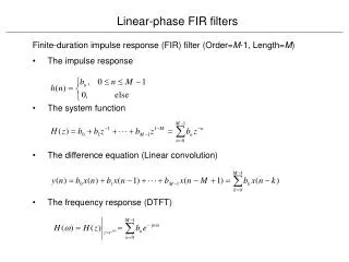
13. Example Find the frequency response of the system with impulse response  t  Reals, h(t) = { 1/3 if t  [0, 3] 0 otherwise EECS 20 Chapter 9 Part 2