Download
1 / 57
570 likes | 713 Views
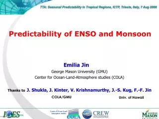
Center of Ocean-Land-Atmosphere studies. TTA: Seasonal Predictability in Tropical Regions, ICTP, Trieste, Italy, 7 Aug 2008. Predictability of ENSO and Monsoon. Emilia Jin George Mason University (GMU) Center for Ocean-Land-Atmosphere studies (COLA).

E N D
Center of Ocean-Land-Atmosphere studies TTA: Seasonal Predictability in Tropical Regions, ICTP, Trieste, Italy, 7 Aug 2008 Predictability of ENSO and Monsoon Emilia Jin George Mason University (GMU) Center for Ocean-Land-Atmosphere studies (COLA) Thanks toJ. Shukla, J. Kinter, V. Krishnamurthy, J.-S. Kug, F.-F. Jin COLA/GMU Univ. of Hawaii
Outline • Current Status of ENSO Predictability in CGCMs • Inherent limits to predictability • Model Flows • Current Status of Monsoon Predictability in CGCMs • Intrasesasonal and seasonal predictability • ENSO-Monsoon relationship • ENSO-Monsoon Relationship in GCM Experiments • Role of tropical Pacific SST anomalies
Model Description and Experimental Design • 1980 – 2004 • 4 case of initial time (Feb, May, Aug, Nov) • 3-15 member • 5-9 months duration • 1980 – 2001 • 4 case of initial time (Feb, May, Aug, Nov) • 9 ensemble member • 6 months duration APCC CLIPAS DEMETER 5 CGCMs 7 CGCMs
What islimitingthe ENSO predictability? • Model Flaws • mean error, phase shift, different amplitude, and wrong seasonal cycle, etc • Flaws in the way the data is used • data assimilation and initialization;chaos within non-linear dynamics of the coupled system • Inherent limits to predictability • some times are more predictable than others; amplitude of SST anomalies with respect toENSO phase • Gaps in the observing system Thanks to Prof. Mark Cane (TTA/ICTP, 2008)
Forecast Skill of NINO3.4 Index Overall Skill Tier-1 MME Forecast ENSO Phase of Initial month SST Intensity of Target month Initial Conditions Feb May Aug Nov El Nino Growth La Nina Growth El Nino Decay La Nina Decay Normal Warm Cold Normal
What islimitingthe ENSO predictability? • Model Flaws • mean error, phase shift, different amplitude, and wrong seasonal cycle, etc • Flaws in the way the data is used • data assimilation and initialization,chaos within non-linear dynamics of the coupled system • Inherent limits to predictability • some times are more predictable than others, amplitude of SST anomalies with respect to ENSO phase • Gaps in the observing system
ENSO Predictability (NINO3.4 index) Annual Cycle Error vs. RMSE Annual Cycle vs. IAV Model Fidelity vs. Skill (a) (c) Intensity of Annual Cycle Error of Annual Cycle Relative Entropy Interannual Variability RMSE ACC • In CGCMs, the intensity of annual cycle and interanual variability show linear relationship. • Models with better climatology tend to have better skill.
Experimental Design • To investigate the property of this model without influence of initial condition, long run simulation is analyzed and compared with forecast data. long run forecast • 1982-2004 period • 9 members • May, Nov IC • 6 months lead • 202-year simulation • Analyzing last 200 years • (200-yr climatology) PRCGC SINTEX-F Luo et al. 2005 • 1981-2003 period • 15 members • 12 calendar months • 9 months lead • 52-year simulation • Analyzing last 50 years • (50-yr climatology) NCEP CFS Saha et al. 2005 Thanks to T. Yamagata and J.-J. Luo (SINTEX-F), and Kathy Pegion (CFS)
NINO 3.4 Index (Observed and CFS) HadSSTv1.1 Calendar year CFS long run
ENSO Characteristics in CFS CGCM Standard Deviation of SST Anomalies over Tropics (a) Observation (c) NINO3 region SST anomalies Calendar Month (b) CFS long run Observation CFS long run Calendar Month Longitude
NINO3 Index in CFS 52-yr simulation Warm minus Cold composite Observation CFS long run SST anomalies Reconstructed data with respect tolead time of 9-month forecast data starting from 12 calendar months(monthly forecast composite) • For observation and forecast, Warm composite (82/83, 86/87, 91/92, 97/98) - Cold composite (84/85, 88/89, 98/99, 99/00) • For CFS 52-yr run, 7 cases for El Nino and 12 cases for La Nina based on one standard deviation definition of DJF Nino3 index
NINO3 Index in CFS 52-yr simulation Warm minus Cold composite Observation CFS long run 1st month 9th month SST anomalies Reconstructed data with respect tolead time of 9-month forecast data starting from 12 calendar months(monthly forecast composite)
Impact of Coupled Model Error on Predictability 1st mode SEOF of SST (Low frequency mode) 1st month 5th month 9th month Obs. long run SINTEX-F MAM NCEP CFS JJA Correlation coefficients with respect to lead month Temporal correlation of PC timeseries with observation Pattern correlation of eigenvector with free long run SINTEX-F NCEP CFS SINTEX-F NCEP CFS Correlation • With increase of the lead month, the forecast ENSO mode progressively approaches to the model intrinsic mode in free coupled run and departs from the observed. Forecast lead month
Model Flaw: Slow Coupled Dynamics This is particular true for a long lead seasonal forecast, because as the forecast lead increases, the model forecast tend to be determined by the model ENSO behavior. Therefore, continuing improvement of the one-tier climate model’s slow coupled dynamics in reproducing a realistic ENSO mode is a key for long-lead seasonal forecast. For example, precipitation forecast depends on accurate forecast of the amplitude, spatial patterns, and detailed temporal evolution of ENSO cycle
RMS Error and Differences between Successive ForecastsNINO3 SST in NCEP CFS forecasts NCEP CFS • Lorenz Curve of Ensemble Mean is not growing • Initial error growth is saturated within two months. • After that, error growth is following the identical model error for all initial cases. For NINO3 index, it will be the error of model ENSO dynamics. • Lorenz Curve of Individual Member grows as fast as Forecast Error. CFS has large ensemble spread due to instability of coupled system. Forecast Error of Ensemble mean Lorenz Curve of Ensemble mean Mean Forecast Error of Each Member Mean Lorenz Curve of Each Member Forecast Error of Each Member Lorenz Curve of Each Member • Forecast error: lower bound of predictability, skill of “current” forecast • Lorenz curve: upper bound of predictability (lower bound of error), growth of initial error defined as the difference between two forecasts valid at the same time (Lorenz 1982)
What islimitingthe ENSO predictability? • Model Flaws • mean error, phase shift, different amplitude, and wrong seasonal cycle, etc • Flaws in the way the data is used • data assimilation and initialization,chaos within non-linear dynamics of the coupled system • Inherent limits to predictability • some times are more predictable than others, amplitude of SST anomalies with respect to ENSO phase • Gaps in the observing system
Different Flavors of El Nino in Nature • Conventional El Niño : “as a phenomenon in the equatorial Pacific Ocean characterized by a positive sea surface temperature departure form normal in the NINO 3.4 region greater than or equal in magnitude to 0.5C averaged over three consecutive months” (NOAA) • Different flavors of El Niño • Trans- Niño (Trenberth and Stepaniak,2001), Dateline El Niño (Lakin and Harrison 2005), El NiñoModoki (Ashok et al. 2007), Non-canonical ENSO (Guan and NIgam, 2008), Warm pool El Niño(Kug et al. 2008), etc. • : Even though there are differences, the distinctive interannual SST variation over the central Pacific which becomes more active in recent year and significantly different global impact form conventional El Niñoare common features. • The transition mechanisms and dynamical structure of two-types of El Nino are significantly different (Kug et al. 2008).
Observed Different Flavors of El Nino Normalized NINO3 and NINO4 SST NINO4 NINO3 Composite of SST (Contour) and Rainfall (Shaded) (1982/83, 1986/87, 1997/98) Mixedl Warm-pool Cold-tongue Either NINO3 SST or NINO4 SST is greater than their standard deviation (1990/91, 1994/95, 2002/03, 2004/05)
Composite of SST Anomalies along the Equator Forecast lead month 7 Shading is for model bias, contour is for observed composite • Composite of seasonal mean SST anomalies • Warm-pool: 4 cases (1990/91, 1994/95, 2002/03, 2004/05) • Cold-tongue: 2 cases (1982/83, 1997/98) Mixed Cold-tongue Warm-pool time CFS SINTEX time
Interannual Variability of NINO3 and NINO4 SINTEX CFS NINO3 NINO3 NINO4 NINO4 Jan Feb Mar Apr May Nov Dec Observed Jun Jul Aug Sep Oct
Scatter Diagram of Normalized DJF NINO3 vs. NINO4 SINTEX CFS Lead month 1 NINO4 Index Lead month 7 NINO3 Index
Relationship between NINO3 and NINO4 SINTEX CFS COR=0.69
Scatter Diagram of Normalized DJF NINO 3 vs. NINO 4 From free long run of two CGCMs SINTEX CFS Obs. 1950-2005 50 years 200 years NINO4 Index NINO3 Index COR=(NINO3, NINO4) 0.69 0.82 0.86 Model Flaw: One Flavor of El Nino
Outline • Current Status of ENSO Predictability in CGCMs • Inherent limits to predictability • Model Flows • Current Status of Monsoon Predictability in CGCMs • Intrasesasonal and seasonal predictability • ENSO-Monsoon relationship • ENSO-Monsoon Relationship in GCM Experiments • Role of tropical Pacific SST anomalies
Background and Objective Observed dominant modes of intraseasonal variability of summer South Asian monsoon (Krishnamurthy and Shukla 2007, 2008) 1. Two intraseasonal oscillatory patterns • 45 and 28-day modes • Their average cycles of variability are correspond to the life cycles of active/break periods of monsoon rainfall over India 2. Two large-scale standing patterns • ENSO mode and Indian Ocean Dipole mode • They persist through out the monsoon season, and seasonal mean monsoon is mainly determined by the two standing patterns. In this study, the space-time evolution of convection over the monsoon region containing the Indian subcontinent, the Indian Ocean, and the Western Pacific and its role on seasonal predictability is investigated in 7 CGCM forecast dataset.
Dominant Modes of Observation Two Standing modes 45-day oscillatory mode Multi-channel singular spectrum analysis • Data: daily OLR anomalies for JJAS 1985-2002 • Region: 40-160E, 20S-35N 28-day Oscillatory mode Power spectra of the space-time principal component • Data: Reconstructed component (RC) which is constructed from the corresponding ST-EOF and ST-PC as the original field • The time length and sequence are exactly those of the original time series (Ghil et al. 2002) Krishnamurthy and Shukla, 2008
Dominant Modes of Observation Standing modes 1st Spatial EOF of daily RC The seasonal mean monsoon is mainly determined by the two standing patterns, without much contribution from the oscillatory modes. ENSO mode IDO mode
Dominant Modes of Observation Oscillatory modes 45-Day 28-Day Composites of eight phases of a cycle of oscillatory mode : Their average cycles of variability are shown to correspond to the life cycles of active and break periods of monsoon rainfall over India.
Dominant Modes of 7 CGCMs Multi-channel Singular Spectrum Analysis • Data: daily rainfall anomalies for JJAS 1981-2002 (only daily climatology is removed.) • Region: 40-160E, 20S-35N • Reference: CMAP pentad rainfall Power spectra of the reconstructed component It shows the dominant standing mode and 45-day mode in one member of each model.
1st EOF of MSSA ENSO mode RC Dominant Modes of 7 CGCMs Standing ENSO mode • They persist through out the monsoon season. • Most of models show indifferent pattern to observed over the Indian continent. • 1st EOF of MSSA RC explains more than 90 % of variance.
Relationship with SST Anomalies Correlation of ENSO mode with daily SST
1st EOF of MSSA Oscillatory mode RC Dominant Modes of 7 CGCMs Oscillatory 45-day mode • It is associated with the life cycles of active and break periods of monsoon rainfall with 45 days period. • Some eastward and northward movements are found to be associated with this oscillatory mode.
Relationship with SST Anomalies Correlation of Oscillatory 45-day mode with daily SST
Role of Intraseasonal Variability on Seasonal Predictability of Indian Monsoon Rainfall ENSO mode IOD mode 45-day mode 28-day mode Oscillatory The strength of the JJAS seasonal mean OLR anomalies is mainly determined by the two persisting standing patterns while the contribution from the oscillatory modes is small. 45-day mode 28-day mode Standing ENSO mode IOD mode Krishnamurthy and Shukla, 2008
Seasonal Predictability of Indian Monsoon Rainfall JJAS Extended IMR Indices of RC Extended IMR: Rainfall over 70-110E, 10-30N
Seasonal Predictability of Indian Monsoon Rainfall JJA Indices - (EIMR index) JJA ACC NINO 3.4 index
Commentary • The most dominant obstacle in realizing the potential predictability of intraseasonal and seasonal variations is inaccurate models, rather than an intrinsic limit of predictability. Thanks to Prof. Jagadish Shukla (TTA/ICTP, 2008)
Outline • Current Status of ENSO Predictability in CGCMs • Inherent limits to predictability • Model Flows • Current Status of Monsoon Predictability in CGCMs • Intrasesasonal and seasonal predictability • ENSO-Monsoon relationship • ENSO-Monsoon Relationship in GCM Experiments • Role of tropical Pacific SST anomalies
ENSO-Monsoon Relationship in GCM Experiments • ENSO-monsoon relationship in NCEP/CFS forecasts • The role of ocean forcing in coupled systems: CGCM vs. “Pacemaker” • The role of air-sea interaction on ENSO-monsoon relationship • Shortcoming in “Pacemaker”: Decadal change of ENSO-Indian monsoon relationship
Regressed field of 1st SEOF of 850 hPa zonal wind Observation 1 Shading: 500 hPa vertical pressure velocity Contour: 850 hPa winds 1 Shading: Rainfall(CMAP and PREC/L) Contour: SST COR (PC, NINO3.4) = 0.85 • From the summer of Year 0, referred to as JJA(0), to the spring of the following year, called MAM(1), a covariance matrix was constructed using four consecutive seasonal mean anomalies for each year. • SEOF (Wang and An 2005) of 850 hPa zonal wind over 40E-160E, 40S-40N • High-pass filter ofeight years • The seasonally evolving patterns of the leading mode concur with ENSO’s turnabout from a warming to a cooling phase (Wang et al. 2007).
Regressed field of 1st SEOF of 850 hPa zonal wind Observation 1 1 Shading: 500 hPa vertical pressure velocity Contour: 850 hPa winds 1 Shading: Rainfall(CMAP and PREC/L) Contour: SST COR (1st PC timeseries of SEOF, N34) Correlation N34 lead N34 lag
Impact of the Model Systematic Errors on Forecasts Pattern Corr. of SEOF Eigenvector • NCEP CFS Retrospective forecast - 15 members • 9 month lead • 1981-2003 (23yrs) Patternl correlation of eigenvector with observation Pattern correlation of eigenvector with free long run Correlation • With respect to the increase of lead month, forecast monsoon mode associated with ENSO is much similar to that of long run, while far from the observed feature. Forecast lead month COR (1st PC timeseries of SEOF, N34) Correlation Observation 1st month forecast 8th month forecast CFS long run N34 lead N34 lag
In CFS coupled GCM, what is responsible to drop the predictability of ENSO – monsoon relationship? • Ocean forcing? • Atmospheric response? • Air-sea interaction? …..
“Pacemaker” Experiments • The challenge is to design numerical experiments that reproduce theimportant aspects of this air-sea coupling while maintaining the flexibility to attempt to simulatethe observed climate of the 20th century. • “Pacemaker”: tropical Pacific SST is prescribed from observations, but coupled air-seafeedbacks are maintained in the other ocean basins (e.g. Lau and Nath, 2003). • Anecdotalevidence indicates that pacemaker experiments reproduce the timing of the forced response to ElNiño and the Southern Oscillation (ENSO), but also much of the co-variability that is missingwhen global SST is prescribed. • In this study, we use NCEP/GFS T62 L64 AGCM.
Pacemaker region Outside the pacemakerregion To handle model drift To merge the pacemaker and non-pacemaker regions Mixed-layer depth “Pacemaker” Experimental Design In this study, the deep tropical eastern Pacific where coupled ocean-atmospheredynamics produces the ENSO interannual variability, is prescribed by observed SST. 165E-290E, 10S-10N No blending Slab ocean mixed-layer Weak damping of 15W/m2/K to observed climatology Zonal mean monthly Levitus climatology
Model and Experimental Design Pacemaker CGCM Atmosphere (GFS T62L64) Atmosphere (GFS T62L64) Local air-sea interaction Fully coupled system Ocean (Full dynamics) SST SST heat flux, wind stress, fresh water flux -γTclim Observed SST heat flux Slab ocean (No dynamics and advection) Mixed layer model + AGCM (1950-2004, 4runs) CGCM (52 yrs)
Definition of Monsoon WNPSMI ISMI EIMR` ISMI WNPSMI m/s mm/4 month • Western North Pacific Summer Monsoon Index (Wang and Fan, 1999) • WNPSMI : U850(5ºN–15ºN, 100ºE–130ºE) minus U850(20ºN–30ºN, 110ºE–140ºE) • Extended Indian Monsoon Rainfall Index (Wu and Kirtman 2004) • EIMR: Rainfall (5ºN–25ºN, 60ºE–100ºE) • ISMI: U850(5ºN–15ºN, 40ºE–80ºE) minus U850(20ºN–30ºN, 70ºE–90ºE)
Lead-lag correlation with Nino3.4 Index WNPSMI EIMR 1st PC timeseries of SEOF ISMI Observation PACE CFS N34 lead N34 lag N34 lead N34 lag Ensemble spread of 4 members of Pacemaker exp.
ENSO Characteristics in CFS CGCM NINO3.4 Index during 1950-2005 (a) Observation (b) CFS CGCM (52 year long run) NCEP CFS has long life cycle of ENSO and associated summer peak. This slow coupled dynamics of model must be responsible for the delay of relationship.
ENSO Characteristics in CFS CGCM Regression of DJF NINO3.4 Index to SST anomalies (a) Observation (b) CFS long run • In CGCM, ENSO SST anomalies show westward penetration with narrow band comparing to the observed.