Query Execution: Architecture, Optimization, and Operators

1. Lecture 22:Query Execution Monday, March 6, 2006

2. Outline • Query execution: 15.1 – 15.5

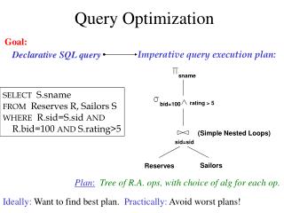
3. Architecture of a Database Engine SQL query Parse Query Logicalplan Select Logical Plan Queryoptimization Select Physical Plan Physicalplan Query Execution

4. Logical Algebra Operators • Union, intersection, difference • Selection s • Projection P • Join |x| • Duplicate elimination d • Grouping g • Sorting t

5. Logical Query Plan T3(city, c) SELECT city, count(*) FROM sales GROUP BY city HAVING sum(price) > 100 P city, c T2(city,p,c) s p > 100 T1(city,p,c) g city, sum(price)→p, count(*) → c sales(product, city, price) T1, T2, T3 = temporary tables

6. Logical Query Plan SELECT P.buyer FROM Purchase P, Person Q WHERE P.buyer=Q.name AND P.city=‘seattle’ AND Q.phone > ‘5430000’ Purchase(buyer, city) Person(name, phone) buyer  City=‘seattle’ phone>’5430000’ Buyer=name Person Purchase

7. buyer  City=‘seattle’ phone>’5430000’ Buyer=name (Simple Nested Loops) Person Purchase (Table scan) (Index scan) Physical Query Plan SELECT S.buyer FROM Purchase P, Person Q WHERE P.buyer=Q.name AND Q.city=‘seattle’ AND Q.phone > ‘5430000’ • Query Plan: • logical tree • implementation choice at every node • scheduling of operations. Some operators are from relational algebra, and others (e.g., scan) are not.

8. Question in Class Logical operator: Product(pname, cname) || Company(cname, city) Propose three physical operators for the join, assuming the tables are in main memory:

9. Question in Class Product(pname, cname) |x| Company(cname, city) • 1000000 products • 1000 companies How much time do the following physical operators take if the data is in main memory ? • Nested loop join time = • Sort and merge = merge-join time = • Hash join time =

10. Cost Parameters The cost of an operation = total number of I/Os result assumed to be delivered in main memory Cost parameters: • B(R) = number of blocks for relation R • T(R) = number of tuples in relation R • V(R, a) = number of distinct values of attribute a • M = size of main memory buffer pool, in blocks

11. Cost Parameters • Clustered table R: • Blocks consists only of records from this table • B(R) << T(R) • Unclustered table R: • Its records are placed on blocks with other tables • B(R)  T(R) • When a is a key, V(R,a) = T(R) • When a is not a key, V(R,a)

12. Selection and Projection Selection s(R), projection P(R) • Both are tuple-at-a-time algorithms • Cost: B(R) Unary operator Input buffer Output buffer

13. Main Memory Hash Join Hash join: R |x| S • Scan S, build buckets in main memory • Then scan R and join • Cost: B(R) + B(S) • Assumption: B(S) <= M

14. Duplicate Elimination Duplicate elimination d(R) • Hash table in main memory • Cost: B(R) • Assumption: B(d(R)) <= M

15. Grouping Grouping: Product(name, department, quantity) gdepartment, sum(quantity) (Product)  Answer(department, sum) Main memory hash table Question: How ?

16. Nested Loop Joins • Tuple-based nested loop R ⋈ S • Cost: T(R) B(S) when S is clustered • Cost: T(R) T(S) when S is unclustered for each tuple r in R do for each tuple s in S do if r and s join then output (r,s)

17. Nested Loop Joins • We can be much more clever • Question: how would you compute the join in the following cases ? What is the cost ? • B(R) = 1000, B(S) = 2, M = 4 • B(R) = 1000, B(S) = 3, M = 4 • B(R) = 1000, B(S) = 6, M = 4

18. Nested Loop Joins • Block-based Nested Loop Join for each (M-2) blocks bs of S do for each block br of R do for each tuple s in bs for each tuple r in br do if “r and s join” then output(r,s)

19. . . . Nested Loop Joins Join Result R & S Hash table for block of S (M-2 pages) . . . . . . Output buffer Input buffer for R

20. Nested Loop Joins • Block-based Nested Loop Join • Cost: • Read S once: cost B(S) • Outer loop runs B(S)/(M-2) times, and each time need to read R: costs B(S)B(R)/(M-2) • Total cost: B(S) + B(S)B(R)/(M-2) • Notice: it is better to iterate over the smaller relation first • R |x| S: R=outer relation, S=inner relation

21. Relation R Partitions OUTPUT 1 1 2 INPUT 2 hash function h . . . M-1 M-1 M main memory buffers Disk Disk Partitioned Hash Algorithms • Idea: partition a relation R into buckets, on disk • Each bucket has size approx. B(R)/M 1 2 B(R) • Does each bucket fit in main memory ? • Yes if B(R)/M <= M, i.e. B(R) <= M2

22. Duplicate Elimination • Recall: d(R) = duplicate elimination • Step 1. Partition R into buckets • Step 2. Apply d to each bucket (may read in main memory) • Cost: 3B(R) • Assumption:B(R) <= M2

23. Grouping • Recall: g(R) = grouping and aggregation • Step 1. Partition R into buckets • Step 2. Apply g to each bucket (may read in main memory) • Cost: 3B(R) • Assumption:B(R) <= M2

24. Partitioned Hash Join R |x| S • Step 1: • Hash S into M buckets • send all buckets to disk • Step 2 • Hash R into M buckets • Send all buckets to disk • Step 3 • Join every pair of buckets

25. Original Relation Partitions OUTPUT 1 1 2 INPUT 2 hash function h . . . M-1 M-1 B main memory buffers Disk Disk Partitions of R & S Join Result Hash table for partition Si ( < M-1 pages) hash fn h2 h2 Output buffer Input buffer for Ri B main memory buffers Disk Disk Hash-Join • Partition both relations using hash fn h: R tuples in partition i will only match S tuples in partition i. • Read in a partition of R, hash it using h2 (<> h!). Scan matching partition of S, search for matches.

26. Partitioned Hash Join • Cost: 3B(R) + 3B(S) • Assumption: min(B(R), B(S)) <= M2

27. External Sorting • Problem: • Sort a file of size B with memory M • Where we need this: • ORDER BY in SQL queries • Several physical operators • Bulk loading of B+-tree indexes. • Will discuss only 2-pass sorting, for when B < M2

28. External Merge-Sort: Step 1 • Phase one: load M bytes in memory, sort M . . . . . . Disk Disk Main memory Runs of length M bytes

29. External Merge-Sort: Step 2 • Merge M – 1 runs into a new run • Result: runs of length M (M – 1) M2 Input 1 . . . . . . Input 2 Output . . . . Input M Disk Disk Main memory If B <= M2 then we are done

30. Cost of External Merge Sort • Read+write+read = 3B(R) • Assumption: B(R)<= M2

31. Duplicate Elimination Duplicate elimination d(R) • Idea: do a two step merge sort, but change one of the steps • Question in class: which step needs to be changed and how ? • Cost = 3B(R) • Assumption: B(d(R))<= M2

32. Grouping Grouping: ga, sum(b) (R) • Same as before: sort, then compute the sum(b) for each group of a’s • Total cost: 3B(R) • Assumption: B(R)<= M2

33. Merge-Join Join R |x| S • Step 1a: initial runs for R • Step 1b: initial runs for S • Step 2: merge and join

34. Merge-Join Input 1 . . . . . . Input 2 Output . . . . Input M Disk Disk Main memory M1 = B(R)/M runs for R M2 = B(S)/M runs for S If B <= M2 then we are done

35. Two-Pass Algorithms Based on Sorting Join R |x| S • If the number of tuples in R matching those in S is small (or vice versa) we can compute the join during the merge phase • Total cost: 3B(R)+3B(S) • Assumption: B(R)+ B(S)<= M2

36. Index Based Selection • Selection on equality: sa=v(R) • Clustered index on a: cost B(R)/V(R,a) • Unclustered index on a: cost T(R)/V(R,a)

37. Index Based Selection B(R) = 2000T(R) = 100,000V(R, a) = 20 • Example: • Table scan (assuming R is clustered): • B(R) = 2,000 I/Os • Index based selection: • If index is clustered: B(R)/V(R,a) = 100 I/Os • If index is unclustered: T(R)/V(R,a) = 5,000 I/Os • Lesson: don’t build unclustered indexes when V(R,a) is small ! cost of sa=v(R) = ?

38. Index Based Join • R S • Assume S has an index on the join attribute • Iterate over R, for each tuple fetch corresponding tuple(s) from S • Assume R is clustered. Cost: • If index is clustered: B(R) + T(R)B(S)/V(S,a) • If index is unclustered: B(R) + T(R)T(S)/V(S,a)

39. Index Based Join • Assume both R and S have a sorted index (B+ tree) on the join attribute • Then perform a merge join • called zig-zag join • Cost: B(R) + B(S)

40. Summary of External Join Algorithms • Block Nested Loop: B(S) + B(R)*B(S)/M • Partitioned Hash: 3B(R)+3B(S); • min(B(R),B(S)) <= M2 • Merge Join: 3B(R)+3B(S • B(R)+B(S) <= M2 • Index Join: B(R) + T(R)B(S)/V(S,a)