Fourier Analyses

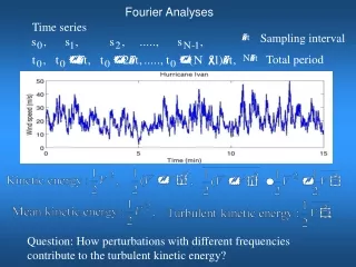
1. Fourier Analyses Time series Sampling interval Total period Question: How perturbations with different frequencies contribute to the turbulent kinetic energy?

2. Decomposition illustration

3. Time-Amplitude domain Frequency-Amplitude domain 10Hz 50Hz 3Hz

4. Wave basics (Euler’s formula)

5. c. Discrete Fourier Transform Observations: N Sampling interval: Period First harmonic frequency: All frequency: nth harmonic frequency: time at kth observation: Time-Amplitude domain Frequency-Amplitude domain If time series F(k) is known, then, the coefficient c(n) can be found as:

6. Forward Transform: Example: Index (k): 0 1 2 3 4 5 6 7 Time (UTC): 1200 1215 1230 1245 1300 1315 1330 1345 Q(g/kg): 8 9 9 6 10 3 5 6 n 0 1 2 3 4 5 6 7 c(n) 7.0 0.28-1.03i 0.5 -0.78-0.03i 1.0 -0.78+0.03i 0.5 0.28+1.03i For frequencies greater than 4, the Fourier transform is just the complex Conjugate of the frequencies less than 4.

7. c(0) =7.0 c(1)=0.28-1.03i c(2)=0.5 c(3)=-0.78-0.03i c(4)=1.0 c(5)=-0.78+0.03i c(6)=0.5 c(7)=0.28+1.03i

8. Aliasing We have ten observations (10 samples) in a second and two different sinusoids that could have produced the samples. Red sinusoidhas 9 cycles spanning 10samples, so the frequency Blue sinusoidhas 1 cycle spanning 10samples, so the frequency Which one is right? Two-point rule Two data points are required per period to determine a wave. 4 observations: 2 waves 2 observations: 1 wave 6 observations: 3 waves N observations: N/2 waves

9. If there were a true signal of f=9 Hz that was sampled at fs=1Hz, then, one would find that the signal has been interpreted as the signal of f=1 Hz. In other words, the real signal f=9 Hz was folded into the signal f=1Hz. This is because the maximum frequency that can be resolved by sampling rate fs=1.0Hz is 0.5 Hz! If sampling rate is , the highest wave frequency can be resolved is , which is called Nyquist frequency

10. Folding Folding occurs at Nyquist frequency. What problem does folding cause?

11. What will cause aliasing or folding? • The sensor can respond to frequencies higher than the rate • that the sensor is sampled. • The true signal has frequencies higher than the sampling rate. How can we remove aliasing? We cannot resolve frequencies higher than Nyquist frequency, i.e., if we have N data points, we can only resolve wave cycles of N/2, but why Fourier transform gives amplitude c(n) up to wave cycle up to n=N-1? C(n) for n>Nf is just the complex conjugate of c(n) for n<Nf. So, half of c(n) for n>Nf gives no new information.

12. Leakage

14. Spectral characteristics (1) Wave with different frequencies

15. (2) Wave frequencies between resolvable frequencies

16. (3) Unresolvable low and high frequencies

17. (4) Red noise

18. (5) Red, white, and blue noise

19. Leakage

20. Multiple waves

21. Fast Fourier Transform (FFT) FFT is nothing more than a discrete Fourier transform that has been restructured to take advantage of the binary computation processes of digital computer. As a result, everything is the same but faster! Relationship between decimal and binary numbers 0 1 2 3 4 5 6 7 8 9 10 0 1 10 11 100 101 110 111 1000 1001 1010 The decimal numbers n and k can be represented by If N=8, then, j=0, 1, 2, 3 7: binary 1 1 1; 5: binary 101; 3: binary 11

22. Energy Spectrum Note that n starts from 1, because the mean (n=0) does not contribute any information about the variation of the signal. For frequencies higher than Nyquist frequency, values are identially equal to those at the lower frequencies. They are folded back and added to the lower frequencies. Discrete spectral intensity (or energy) Spectral energy density

23. Example Index (k): 0 1 2 3 4 5 6 7 Time (UTC): 1200 1215 1230 1245 1300 1315 1330 1345 Q(g/kg): 8 9 9 6 10 3 5 6

24. N observations

25. Graphical presentation of atmospheric turbulence spectra Linear-linear presentation Semi-log presentation Log-log presentation Log(fS(f)) vs. log(f)

26. Blackhar Window: N=9000

27. Turbulent spectral similarity • Energy associated with large-scale • motion eventually is transferred to • the large turbulent eddies. • The large eddies then transport this • energy to small-scale eddies. • These smaller scale eddies then • transfer the energy to even • small-scale eddies..., and so on • Eventually, the energy is dissipated • into heat via molecular viscosity. Inertial sub-range: An intermediate range of turbulent scales that is smaller than the energy-containing eddies but larger than viscous eddies. In the inertial subrange, the net energy coming from the energy-containing eddies is in equilibrium with the net energy cascading to smaller eddies where it is dissipated.

28. Kolmogorov's Energy Spectrum Inertial sub-range is in an equilibrium state, Kolmogorov assumes that the energy density per unit wave number depends only on the wave number and the rate of energy dissipation. wavelength wave-number 3 3 5 5

29. 2D FFT . Let χ(m,n) be a generic scalar on a 2D grid, where m=0,1,…,M-1; n=0,1,…N-1 are the grid number index; and M and N are the number of grids in x and y direction, the 2D-FFT of χ(m,n), then, may be written as, where k and l are the 2D-FFT wavenumber index in x and y direction, and are the angular wavenumber in x and y direction. χ(m,n), then, can be reconstructed as Spectral energy can be written as Again, energy is conserved

30. Project 2 . Using 1D FFT to decompose the provided hurricane data in terms of wavenumbers.