Download

1 / 81
1.1k likes | 2.53k Views
Fourier Series ,Fourier Integral, Fourier Transform. Group #9 Yizhi Hong Jiaqi Zhang Nicholas Zentay Sagar Lonkar. 17.1 Introduction. Main Work : Théorie analytique de la chaleur (The Analytic Theory of Heat)

E N D
Fourier Series ,Fourier Integral, Fourier Transform Group #9 Yizhi Hong Jiaqi Zhang Nicholas Zentay SagarLonkar
17.1 Introduction • Main Work: • Théorieanalytique de la chaleur • (The Analytic Theory of Heat) • Any function of a variable, whether continuous or discontinuous, can be expanded in a series of sines of multiples of the variable (Incorrect) • The concept of dimensional homogeneity in equations • Proposal of his partial differential equation for conductive diffusion of heat • Discovery of the "greenhouse effect" Jean Baptiste Joseph Fourier (Mar21st 1768 –May16th 1830) French mathematician, physicist http://en.wikipedia.org/wiki/Joseph_Fourier
17.2 Even, Odd, and Periodic Functions even function: odd function: some characteristic: even+even=even even*even=even odd+odd=odd odd*odd=even even*odd=odd If f is even, then If f is odd, then
Every function can be uniquely decomposed into the sum of an even function, say fe, and an odd function, say fo. Periodic function for every x in the domain of f. Then we say that f is a periodic function of x, with period T. And f is T-periodic.
Examples: Even function : Cosine function i.e. cos(θ) Odd function: Sine function i.e. sin(θ) Periodic Function: Both sine and cosine functions are periodic with a period of 2 π
17.3 Fourier Series of a Periodic Function If f(x) is periodic, of period 2l, then we define the Fourier series of f, say FS f, as Where the coefficients are given by the Euler formulas,
For FS f to represent f we need the series to converge, and we need its sum function to be the same as the original function f(x).
THEOREM 17.3.1 Fourier Convergence Theroem Let f be 2L-periodic, and let f and f ‘ be piecewise continuous on [-L,L]. Then the Fourier series converges to f(x) at every point x at with f is continuous, and to the mean value [f(x+)+f(x-)]/2 at every point x at which f is discontinuous. where h→0 through positive values. If f(x+)=f(x-)=f(x), then f is continuous at x, otherwise it is discontinuous.
Even and odd And
For the reason that: for |c1|≠|c2|. for |c1|≠|c2|. for |c1|≠|c2|.
Example: The function given by: y=-x - π≤x≤0 y=x 0≤x≤ π The period of the above function is 2π. Thus 2l = 2π Therefore l= π
= = 0 + n=0 FS f n=1 FS f n=2 FS f n=3 FS f n=4 FS f n=5 FS f
s1 s0 s3 s5
Example:Periodically forced oscillation: mass-spring system m = mass c = damping factor k = spring constant F(t) = 2L- periodic forcing function mx’’(t) + cx’(t) + k x(t) = F(t) m F(t) k http://www.jirka.org/diffyqs/ Differential Equations for Engineers
The particular solution xp of the above equation is periodic with the same period as F(t) . The coefficients are k=2, and m=1 and c=0 (for simplicity). The units are the mks units (meters-kilograms- seconds). There is a jetpack strapped to the mass, which fires with a force of 1 newton for 1 second and then is off for 1 second, and so on. We want to find the steady periodic solution. The equation is: x’’ + 2x = F(t) Where F(t) => 0 if -1<t<0 1 if 0<t<1
To find the particular solution we take x = A cos(nt) + Bsin(nt) x’ = - nAsin(nt)+ nBcos(nt) x’’ = - n22x x’’ + 2x = sin(nt) (2- n22)x = sin(nt) x = Particular solution corresponding to ½ is given by (2- n22)x = ½ at n=0 Thus x = ¼
Thus the desired steady state response is, by linearity and superposition, xp = Plot of steady periodic solution thus obtained is:
Complex exponential form for Fourier series Using the definitions and it is possible to re-express the Fourier series formula in terms of complex exponentials, as follows: where
Although the cn's and exponentials in FS f are complex, the series does have a real-valued sum. The usual definition does not apply because the lower limit is infinite as well. It can be shown that the appropriate meaning of the above series is
With this we can proceed: Changing n to -n for the second sum gives:
For n = 0, , For n > 0, , For n < 0,
Example: Find the Fourier series for the function defined by Solution: Where Reference: Fourier Analysis (Author: Eric State, Pure and Applied Mathematics: a Wiley-Interscience Series of Texts, Monographs, and Tracts ) P 11
We’ll compute the cn(f) first, we get So We also have and so
17.4 Half- and Quarter- Range Expansions It often happens in applications, especially when we solve partial differential equations by the method of separation of variables, that we need to expand a given function f in a Fourier series, where f is defined only on a finite interval. We define an “extended function”, say fext, so that fext is periodic in the domain of -∞< x < ∞, and fext=f(x) on the original interval 0<x<L. There can be infinite number of such extensions. Four extensions: half- and quarter- range cosine and sine extensions, which are based on symmetry or antisymmetry about the endpoints x=0 and x=L.
1.HRC (half range cosines) fextis symmetric about x=0 and also about x=L. Because of its symmetry about x=0, fext is an even function, and its Fourier series will contain only cosines, no sines. Further, its period is 2L, so L is half the period. , ( 0< x < L)
Proof: For the half-range cosine case the period is 2L, and , , .
2.HRS (half range sines) fextis antisymmetric about x=0 and x=L, the period is 2L, and we have the half-range sine extension. , ( 0< x < L)
3.QRC (quarter range cosines) fext is symmetric about x=0 and anti-symmetric about x=L, the period is 4L (so L is only a quarter of the period), and we have the quarter-range cosine extension. , ( 0< x < L) .
4.QRS (quarter range sines) fext is anti-symmetric about x=0 and symmetric about x=L, the period is, and we have the quarter-range sines extension. , ( 0< x < L) .
Example: F(x) = sin(x) 0<x<π L= π HRC: = = ( 0< x < )
HRS: , ( 0< x < L) = 0 for n>1 ( 0< x < )
QRC: , ( 0< x < L) = ( 0< x < )
QRS: , ( 0< x < L) ( 0< x < )
17.5 Manipulation of Fourier Series Uniform convergence
THEOREM 17.5.1Weierstrass M-Test If is a convergent series of positive constants and ||≤ on an x interval I, then is uniformly (and absolutely) convergent on I. THEOREM 17.5.2Termwise Differentiation of Series Let converge on an x interval I. Then , if the series on the right converges uniformly on I.
THEOREM 17.5.3 Uniqueness of Trigonometric Series If , Where the trigonometric series on the left- and right-hand sides converge to the same sum for all x, then a0=A0, an=An, and bn=Bn for each n. THEOREM 17.5.4Termwise Integration of Fourier Series If a Fourier series is integrated termwise between any finite limits, the resulting series converges to the integral of the periodic function corresponding to the original series.
Example: Verify the convergence of the series on the given interval: on 2<x<5 By WeierstrassM-test: an(x) = ≤ ≤ on 2<x<5 is a convergent geometric series. Therefore the given series is a convergent on the given interval.
17.6 Vector Space Approach Some definitions: • Function spaceCp[a,b] of all real-valued piecewise-continuous functions defined on [a,b]. • f=f(x) and g=g(x) be any two functions in Cp[a,b], and let α be any (real) scalar. f + g ≡f(x) + g(x), αf≡α f(x). Observe that if f and g are piecewise continuous on [a,b] then f+gand αfare also piecewise continuous, so Cp[a,b] is closed under vector addition and scalar multiplication. • We define the zero vector 0 as the function which is identically zero, so that f + 0 = f(x) + 0 = f
We define the negative inverse of f = f(x) as –f≡ -f(x), in which case we have f + (-f) = f(x) + [-f(x)]=0 = 0 • Inner product for Cp[a,b], the inner product of f and g as . f and g are orthogonal if <f,g>=0, that the norm ||f|| is defined as , and f is said to be normalized if ||f||=1. • is ON (orthonormal ) set in S, then the best approximation of f within span is given by the orthogonal projection of f onto span , namely, by
To apply these results to Fourier series, let S be Cp[a,b], with the inner product and norm defined above, let a=-L and b=L, and consider the vectors e1=1, e2=, e3=, … , e2k=, e2k+1=in Cp[-L,L]. is orthogonal by virtue of the inner product definition and the integrals:
So that the normalized en’s are: Thus we can approximate a givenf=f(x), in Cp[a,b], in the form:
THEOREM 17.6.1 Vector Convergence If f(x) is piecewise continuous on [-L,L] and a0, a1, b1, a2, b2, … are the Fourier coefficients, then Holds in the sense of vector (least-square) convergence, namely,
Example: Find the error for the following function: F(x) = defined on the interval –π<x<π ||E||2= l=π for n= odd = 0
||E||2 = = K ||E||2 ||E|| 1 0.0747 0.27 2 0.0747 0.27 3 0.0118 0.11 4 0.0118 0.11 5 0.0037 0.06 6 0.0037 0.06 7 0.00150.04 The error goes on decreasing as k increases.
THEOREM 17.7.1 Sturm-LiouvilleTheorem Let and denote any eigenvalue and corresponding eigenfunction of the Sturm-Liouville eigenvalue problem (1), respectively. (a). The eigenvalues are real (b). The eigenvalues are simple. That is, to each eigenvalue there corresponds only one linearly independent eigenfunction. Further, there are an infinite number of eigenvalues, and they can be ordered so that where . (c). Eigenfunctions corresponding to distinct eigenvalues are orthogonal. That is, if , then . (d). Let f and f' be piecewise continuous on a≤x≤b. If , then the series converges to f(x) if f is continuous at x, and to the mean value [f(x+)+f(x-)]/2 if f is discontinuous at x, for each point x in the open interval a < x < b.
Example: Solve the Sturn-Liouville problem There a is a constant in the interval (0,1). Also write down the expansion of an arbitrary element of the appropriate “ ” space in terms of the eigenfunctions of the problem. Solution: We put and So Whose general solution is if not Reference: Fourier Analysis (Author: Eric State, Pure and Applied Mathematics: a Wiley-Interscience Series of Texts, Monographs, and Tracts ) P 224