Download
1 / 52
520 likes | 619 Views
Central Arizona Water Demand Model Water Resources Development Commission Scenarios. March 29, 2010. Central Arizona Water Demand Model Area. AMA/Model Boundary. Supply/Demand Distribution. Supply. Demand. Primary Objectives: Model Design.

E N D
Central Arizona Water Demand ModelWater Resources Development Commission Scenarios March 29, 2010
Central Arizona Water Demand Model Area AMA/Model Boundary Supply/Demand Distribution Supply Demand
Primary Objectives: Model Design • Develop dynamic, population-driven demand projections for municipal, industrial, and agricultural uses • Various growth scenarios & conservation rates • Project demand/supply at the AMA level to avoid inter-AMA “peanut butter” effect of previous studies • Project available surface water, groundwater, effluent, and other supply categories based on existing regulations and priorities • Address major regulatory tradeoffs/outcomes such as overdraft • Model multiple interrelationships between supply, demand and storage categories • Incorporate category-specific restrictions on water use and availability • Project likely demand for new imported supplies
Primary Modeling Assumptions • Supply and demand in the Phoenix, Pinal, and Tucson AMAs are each modeled separately • Projected local demand in each AMA (municipal, industrial, agricultural use) • Projected local supplies in each AMA (groundwater, surface water, effluent, and storage/recovery) • Local supplies in one AMA are NOT available to other AMAs • M&I demand above locally-available supply assumed to be met via direct utilization of CAP water under M&I subcontracts, or else by incurring groundwater replenishment obligations (CAGRD) • Once demand above local supply exceeds available M&I and CAGRD pools, results in demand for “new imported supply” • Agricultural demand does not directly result in demand for imported supply, although agricultural uses may consume local renewable supplies that might otherwise be available for M&I use • Example: when CAP NIA pool eliminated in 2030, agricultural users revert to groundwater
Primary Data Sources • ADWR historic data for municipal, industrial, agricultural demand and reported surface water, groundwater, and effluent use • ADWR maintains detailed post-1985 records by user and by category • ADWR Fourth Management Plan Assessment 2010-2025 projections • Currently in near-final draft; Tucson AMA published • Based on detailed, provider-by-provider reporting and surveys • Used for 2010-2025 projections in some circumstances; also used to calibrate regression models and overall model results • Arizona Lower Basin Depletion Schedule (ADWR) • CAP Subcontractor Report, priority schedule, and delivery data • Indian settlement agreements • Water provider data • City of Phoenix, City of Tucson, MAG water/wastewater use data
Modeling Scenarios • For the initial set of WRDC scenarios, focused on three primary variables: • Population growth rates (6 WRDC scenarios plus DES) • Water conservation rates (Basin Study “Target” & “Low GPCD”) • Available CAP diversions (Basin Study “Tribal” vs. ADWR minimum) • These variables have the greatest impact on local demand growth and the timing and potential volume of future Colorado River demand • Because of complex interrelationships between supply/demand categories, can produce counter-intuitive results • Alternative scenarios involving reuse rates, agricultural retirement, and storage recovery strategies should be explored
Projected municipal use based on AMA projected population times an aggregate GPCD, plus urban irrigation/turf AMA populations based on WRDC population scenarios Aggregate GPCD for study period calculated based on water use targets for primary municipal categories Municipal conservation rates in model tracked via GPCD rates for indoor water use and GPHUD rates for exterior water use independent rates for pre-2000 residential, post-2000 single-family residential, post-2000 multi-family residential, and non-residential (commercial & industrial) uses “Target” GPCD (baseline for Basin Study) utilizes ADWR Third Management Plan requirements Existing (pre-2000) residential (122 GPCD interior/exterior) New single-family residential (57 interior, 128-178 exterior) New multi-family residential (57 interior, 77 – 78 exterior) Non-residential baseline (63 GPCD) includes all industrial and commercial uses supplied directly by municipal providers under TMP guidelines Municipal Use
Low GPCD Scenario • Also introduced high conservation effort “Low GPCD” scenario to demonstrate effects on very high populations in WRDC scenarios • GPCD reductions on logarithmic curve • Starting from current provider-reported GPCD rates • Achievement of Third Management Plan (TMP) targets by 2020 • Achievement of Western Resource Advocates (WRA)-recommended targets by 2035-2040 • Diminishing rates of conservation improvement thereafter
Water Conservation Scenarios 2009 Levels
Municipal Use: Urban Irrigation • Urban irrigation (surface water) based on recent historic data and projected conversion • SRP service area (Phoenix AMA): assumes continuation of current deliveries for turf/landscaping uses • Maricopa-Stanfield (Pinal AMA): conversion of surface water inside MSIDD boundaries based on MSIDD data • Urban turf facility use (reclaimed water) based on recent GPCD rates under Third Management Plan guidelines (ADWR projection) • Varies by AMA (between 8 – 15 GPCD)
Industrial use (i.e., industrial uses not supplied by municipal providers) projected based on five primary categories of current self-supplied industrial uses Population-driven models developed for largest use categories (turf & electric) Major categories Turf facilities (golf, recreation, playing fields) Population-based regression model based on historic data Electrical generation (see below) Mining use (including exchange) – ADWR survey Dairy (including CAFO) – ADWR survey; assumes relocation to rural areas over time Other (sand & gravel, remediation, heavy industry) – ADWR survey Industrial Use
Industrial Use: Electrical • Electrical generation use model developed with assistance from Arizona Public Service: • MWh per capita per year • Gallons per MWh • Statewide thermal generation • AMA percentage share of thermal energy generation • Baseline assumptions built from EIA data sets • Variables can be adjusted to reflect greater/lesser energy use, water use efficiency, and geographic distribution of generation • Model does not currently address energy requirements associated with increased Colorado River diversions
Agricultural use assumed not to directly generate new demand for renewable supply – but may indirectly result in new demand by preventing access to renewable supplies NIA agricultural use projected based on utilization of IGR-entitled acres Generally assumes continuation of Third Management Plan efficiencies Indian and non-Indian agricultural uses projected separately NIA projected to continue to decline in all 3 AMAs as a result of conversion of IGR acreage to municipal use Most farmland eliminated in Phoenix and Tucson AMAs by end of study period No new non-Indian irrigated acreage in AMAs Indian agriculture projected to stabilize by 2025 (see below) CAP NIA pool eliminated by 2030, following current schedule NIA pool users assumed to convert to groundwater use Agricultural Use
Agricultural Use Projections • Regression models developed specific to each AMA based on historic data; calibrated/checked against ADWR survey data in Assessments • Pure population based models, urban land conversion, and population density-based models all explored • Selected model uses hybrid approach; predicts farmland conversion based on historic relationship of post-1985 population growth to total loss of irrigated acres • Result: declining rate of conversion as low-value farmland used up and urban boundaries expand into desert areas • In Phoenix AMA, waterlogged/non-waterlogged areas projected separately • Waterlogged acreage declines more slowly due to high development constraints • Utilization rates for irrigated acres and farm water duties based on recent reported data and precipitation rates • No adjustment for aquifer declines or projected increases in pumping costs • Model also accounts for canal losses based on historic data/trends
Indian build-out of current CAP entitlements by 2025 for planned agricultural uses, with constant rates of use thereafter Indian groundwater use based on ADWR projections (from tribal planning documents) Direct use of CAP and build-out schedules based on current CAWCD/ADWR projections for Indian use Indian municipal/industrial uses assumed to be washed out in AMA M&I projections Indian leasing assumes that all settlement-authorized, implemented leases of CAP water occur with partial future use of all settlement-authorized leases (approximately 170 kaf total) Leases counted as Indian priority utilization of CAP (but reduce demand for new imported supply) Indian Use & Leasing
CENTRAL ARIZONA WATER SUPPLY MODEL Verde Salt Upper Gila SRP Storage (Roosevelt) SRP Storage (Horseshoe) San Pedro Colorado River Butler San Carlos Agua Fria SRP McMullen CAP Pleasant Phoenix AMA Pinal AMA Tucson AMA Harquahala Phoenix Basin Pinal Basin Tucson Basin GW Inflow/ Outflow GW Inflow/ Outflow GW Inflow/ Outflow CAGRD Santa Cruz Lower Gila
Surface Water • Available surface water based on historic average availability from primary surface water sources • Salt River Project (Salt & Verde) normal flows (PHXAMA, on-Project) • SRP gatewater (PHXAMA, off-Project) • Plan 6 SRP storage (PHXAMA, off-Project) • Agua Fria (PHXAMA, MWD service area) • Gila (PAMA, SCIDD service area) • Santa Cruz (underflow to TAMA only) • All surface water assumed to be available to M&I unless used by agricultural users • Conversion of agricultural surface water use modeled based on regression of historic agricultural surface water use against loss of irrigated acres • Indian surface water assumed to be unavailable for NI uses
Reclaimed Water • Effluent generation rates based on City of Phoenix, Tucson pre- and post-2000 effluent generation rates for residential and non-residential users • 100% of post-2000 SF/MF interior use (losses offset by stormwater infiltration) plus percentage of pre-2000 residential and NR use • Provides effluent generation feedback for water conservation assumptions • Model assumes partially “closed system” with portion of effluent consumed by urban direct use (turf), agricultural direct use, and industrial use • Portion allocated to loss/downstream discharge (Gila, Santa Cruz) based on calibration of projected supply to accounted-for effluent use and “downhill” geographic location of primary wastewater generation • For calibration, recent storage data compared to reported 91st Ave, 27th Ave, and Pima County regional WWTP discharges/downstream diversions & projected total capacity
Effluent Storage and Recovery • After subtracting projected direct use and discharge, remainder of effluent allocated to storage • Under baseline conditions, all effluent associated with post-2010 growth is allocated to storage use • Assumes no new downstream losses • Results in rapidly increasing accruals to aquifer storage • Managed/constructed USF, GSF facilities for LTSC generation or annual storage/recovery • Allocation between annual storage/recovery and long-term storage changes over time based on historic trends • Direct effluent use prohibited by ADEQ rules; however, ASR effluent storage treated as direct M&I supply that offsets demand for renewable supplies • Increased ASR allocation could be used to offset new demand for imported supply or to offset assumption of increased downstream discharge (at the cost of reductions to net overdraft)
CAP Storage and Recovery • Available CAP excess water allocated to managed/ constructed USF and GSF facilities • Storage assumed to continue as long as CAP excess water is available above NIA and/or GRD pools • Distribution pursuant to “storage model” distributing CAP excess among AMAs and between managed USF, constructed USF, and GSF facilities based on historic trends • Under baseline assumptions, aside from GRD pool water, no CAP water is allocated to ASR • Results in substantial accumulation of LTSCs during early portion of study period • Accumulated LTSCs are assumed to be available to offset/mitigate shortage conditions and/or groundwater overdraft • Model tracks LTSC generation, accumulation, and recovery to provide running total balance of accumulated LTSCs from CAP and effluent storage • Totals can be compared against cumulative shortage and overdraft values
M&I Groundwater Use • Calculation of available groundwater supply for M&I use based on current Groundwater Management Act requirements • To calculate supply, model tracks availability of groundwater not subject to replenishment obligations pursuant to GMA • Excess groundwater use subject to replenishment treated as demand for imported supply (CAGRD obligation) • Baseline assumes no regulatory changes to address overdraft conditions • Model projects that all AMAs fail to reach safe yield within study period • M&I groundwater use projected based on combination of: • Pre-1995 undesignated provider use (exempt from GMA) • DAWS/CAWS groundwater allowance use • Extinguishment credits • Exempt wells & domestic exempt providers • Industrial groundwater (GIUs and grandfathered rights)
DAWS Allowance Modeling • Groundwater allowances provide for authorized, one-time groundwater mining by providers to serve development uses • DAWS/CAWS split based on historic trends in each AMA • Initial DAWS allowance use based on recent and planned provider use • Designated providers assumed to consume 100% of balances by 2110, DAWS allowance use assumed to grow based on 4% incidental recharge • Debits/credits against available groundwater allowance account beginning from 2010 accumulated balances • Pinal AMA has annualized allowances based on 2007 DAWS populations • 2007 service populations at 125 GPCD, plus undesignated providers that convert by 2010 • Additional “transition volume” of 0.35 af per residential lot served by 2010, calculated based on new CAWS population adjusted by census PPHU
CAWS Allowance Modeling • CAWS allowance use based on post-1995 CAWS populations • Available allowances based on incremental increase in demand multiplied by GMA allowance schedule (decreases to zero by end of 5th Management Plan) • Extinguishment credits accrue to groundwater allowance accounts based on historic and projected irrigated acreage loss multiplied by extinguishment credit schedule (decreases to zero by 2025 in Phoenix/Tucson, 2051 in Pinal) • Once allowances are exhausted, development assumed to shift to renewable supply (either directly or via CAGRD replenishment obligations) • Results in “peak” allowance use sometime after 2030 • Pinal AMA differentiates between pre- and post-2007 CAWS developments due to 2007 AWS rule changes • 2007 developments receive 125 GPCD annualized allowance; post-2007 developments receive one-time allowance based on GMA allowance schedule • Pre-2007 “annualized” extinguishment credits assumed to support 100% annualized 2007 CAWS use
Other Groundwater Supplies • Pre-1995 undesignated providers assumed to continue exploitation of GMA exemptions • Exempt well growth modeled based on log regression against population • Consistent with declining rate of growth in exempt well use over time due to urban expansion (exempt wells rarely permitted in in-fill locations) • Domestic exempt provider use based on linear regression of exempt population against AMA populations • Industrial groundwater use projected based on historic distributions of GIU/grandfathered right use versus renewable supplies • Industrial use assumed to remain heavily dependent on groundwater consistent with GMA loopholes • Regulatory changes widely anticipated; could result in substantial redistribution of future industrial demand to renewable supplies
Agricultural Groundwater Use • Agricultural groundwater use assumed to be “supply of last resort” due to heavily-subsidized agricultural access to renewable supplies • All IGR acres are assumed to have access to groundwater as secondary supply • Available surface water, CAP NIA water, CAP GSF storage, effluent GSF storage, and effluent direct use subtracted from total agricultural use • Agricultural groundwater use increases significantly following loss of CAP NIA pool supplies • Under baseline assumptions, overall groundwater use declines substantially due to high rates of agricultural conversion
Recharge & Overdraft Modeling • Model balances municipal, industrial, and agricultural groundwater withdrawals and modeled groundwater basin outflows against natural and artificial recharge sources to calculate net annual overdraft in each AMA • Provides “closed system” feedback from changes in water utilization • Recharge based on Assessment data/projections • Mountain front recharge (historic data) • Direct infiltration/streambed recharge from precip (historic data) • Groundwater inflow/outflow balance (ADWR regional models) • Incidental recharge (as percentage of municipal, industrial (turf), and agricultural uses/canal losses • “Cuts to the aquifer” from LTSC generation • Note that “paper” overdraft exceeds actual (current) overdraft due to LTSC accounting
Storage and Overdraft Tradeoffs • New Colorado River demand under each of these scenarios could theoretically be offset by increased levels of direct reuse (instead of committing effluent to storage) • Under CRC selected scenario, 14.6 million acre-feet of cumulative storage during the study period • However, critical to note that there is a direct tradeoff between direct reuse rates and groundwater overdraft • Model suggests heavy groundwater overdraft through most of the study period • Under CRC selected scenario, 21.2 million acre-feet of cumulative overdraft over the study period, but net annual overdraft is finally controlled by effluent storage near the end of the study period (safe-yield achieved) • If higher direct use rates were introduced, groundwater overdraft would continue • Recharge of effluent causes AMAs to achieve safe-yield in higher growth scenarios
Colorado River Build-Out Schedules • Colorado River build-out schedules define the amount of non-CAP use of Colorado River water by users along the Colorado River mainstem (agricultural users, on-river municipalities, and Indian tribes) • CAP effectively has the lowest priority to Colorado River water (post-1968 = Priority 4), shared with approximately 157,000 acre-feet of other on-River users • CAP is the “cleanup” user; receives all “surplus” water not utilized by same priority or higher-priority users (allowing excess diversions above 1.5 maf) • Surplus diversions allow for potential continued existence of CAP excess pool after CAP subcontracts built out to full 1.415 maf (1.5 maf less evaporation loss) • CAP bears 90% of the risk of any shortage to Priority 4 entitlements • Chosen Colorado River use scenarios • Tribal CR Buildout (Basin Study baseline): ADWR projections for on-river users except for Indian tribes; Indian tribes build out to near-full capacity based on 2010 tribal schedules. • Minimum CR Use (ADWR projections): Only modest increases in use of existing entitlements based on current ADWR projections; little additional use by CRIT, YMIDD, or Fort Mohave; CAP continues to receive diversions in excess of 1.5 maf (ADWR projections)
Net Demand for New Imported Supply • Available CAP diversions based on Arizona side Lower Basin Depletion Schedule • Baseline assumes “partial buildout” of mainstem entitlements (i.e., Indian and Yuma area uses do not exceed recent levels) • Based on ADWR-developed schedule for AWBA planning purposes • CAP system evaporation/loss based on historic 5% of total diversions • Net available CAP water divided into: (1) Priority 3 Colorado River (Indian settlement transfers), (2) M&I priority subcontract, (3) Indian priority subcontract, (4) NIA M&I allocation, (5) NIA Indian allocation, and (6) excess “pools” • To the extent that modeled demands within M&I categories exceed available pools, results in net “unmet” demand (demand for new imported supply) • “Unmet” demand can be offset by Indian lease (reallocation of Indian pool water) and/or imported groundwater (or change in AMA water use) • Remainder assumed to be new Colorado River demand
M&I Subcontract Pool Allocations • M&I demand for imported supply in each AMA is divided between an “M&I subcontract pool” (composed of both M&I priority subcontracts and NIA priority subcontracts/future allocations) and a “CAGRD pool” based on historic/projected trends • NIA water that will be available for future allocation that is not already associated with the Indian settlement pool is assumed to be allocated for M&I use in the future • “CAGRD pool” translates into 3-AMA demand for CAP/imported supply to meet groundwater replenishment obligations (see below) • “M&I subcontract pool” demand grows inside the total volume of CAP M&I subcontracts in each AMA • Provider-based distribution; unallocated CAP water and ASLD subcontracts assumed to be allocated proportionately among AMAs based on current distribution ratios • To the extent that M&I subcontract demand is less than the available M&I subcontract pool, results in available excess water • If M&I subcontract demand exceeds the available pool, results in “unmet” demand (demand for new imported supply)
Indian Pool Allocations • Indian demand grows inside of “Indian subcontract pool” composed of Indian priority, transferred Colorado River water, and reallocated NIA priority CAP water • Pool includes unallocated settlement pool water (assumes allocated to Indian users within the study period) • To the extent Indian demand schedule falls below available pool, results in excess CAP water • Priority 3 water that has been reallocated to municipal users is treated as Indian lease water • Baseline assumes near build-out of Indian demand by 2030 • Indian leases included in Indian demand schedule • Inclusion of leases reduces available excess water, but lease water is available to offset net “unmet” M&I and CAGRD demands • Indian demand is assumed to be limited to available Indian pool; Indian demands do not necessarily generate new demand for imported supply • However, model tracks shortfalls to Indian pools for reporting purposes
Excess Pool Allocations • Excess pool composed of excess M&I subcontract, Indian subcontract, and CAP diversions above M&I and Indian long-term subcontract entitlements • Excess pool assumed to be allocated between NIA, CAGRD, and storage use • NIA pool has first priority for excess water; agricultural NIA contracts expire progressively in 2017, 2024, and 2030 • CAGRD pool has second priority; limited to 35,000 af per 2009 “Access to Excess” rules and CAP-sponsored legislation • To the extent CAGRD pool demand exceeds 35,000 af, results in “unmet” demand (demand for new imported supply) • After subtraction of NIA and CAGRD uses, remaining excess water allocated to “storage model” and allocated to USF/GSF facilities as detailed above • Model assumes 100% utilization of available CAP diversions