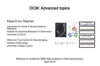
DCM: Advanced topics

1. DCM: Advanced topics Klaas Enno Stephan Laboratory for Social & Neural Systems Research Institute for Empirical Research in Economics University of Zurich Wellcome Trust Centre for Neuroimaging Institute of Neurology University College London Methods & models for fMRI data analysis in Neuroeconomics, April 2010

2. Overview • Bayesian model selection (BMS) • Nonlinear DCM for fMRI • Integrating tractography and DCM

3. Pitt & Miyung (2002) TICS Model comparison and selection Given competing hypotheses on structure & functional mechanisms of a system, which model is the best? Which model represents thebest balance between model fit and model complexity? For which model m does p(y|m) become maximal?

4. Bayesian model selection (BMS) Model evidence: Gharamani, 2004 p(y|m) y all possible datasets accounts for both accuracy and complexity of the model Model comparison via Bayes factor: allows for inference about structure (generalisability) of the model • Various approximations, e.g.: • negative free energy, AIC, BIC Penny et al. 2004, NeuroImage Stephan et al. 2007, NeuroImage

5. Approximations to the model evidence in DCM Maximizing log model evidence = Maximizing model evidence Logarithm is a monotonic function Log model evidence = balance between fit and complexity No. of parameters In SPM2 & SPM5, interface offers 2 approximations: No. of data points Akaike Information Criterion: Bayesian Information Criterion: AIC favours more complex models, BIC favours simpler models. Penny et al. 2004, NeuroImage

6. Bayes factors To compare two models, we can just compare their log evidences. But: the log evidence is just some number – not very intuitive! A more intuitive interpretation of model comparisons is made possible by Bayes factors: positive value, [0;[ Kass & Raftery classification: Kass & Raftery 1995, J. Am. Stat. Assoc.

7. The negative free energy approximation • Under Gaussian assumptions about the posterior (Laplace approximation), the negative free energy F is a lower bound on the log model evidence:

8. The complexity term in F • In contrast to AIC & BIC, the complexity term of the negative free energy F accounts for parameter interdependencies. • The complexity term of F is higher • the more independent the prior parameters ( effective DFs) • the more dependent the posterior parameters • the more the posterior mean deviates from the prior mean • NB: SPM8 only uses F for model selection !

9. M3 attention M2 better than M1 PPC BF 2966 F = 7.995 stim V1 V5 M4 attention PPC stim V1 V5 BMS in SPM8: an example attention M1 M2 PPC PPC attention stim V1 V5 stim V1 V5 M3 M1 M4 M2 M3 better than M2 BF 12 F = 2.450 M4 better than M3 BF 23 F = 3.144

10. Fixed effects BMS at group level Group Bayes factor (GBF) for 1...K subjects: Average Bayes factor (ABF): Problems: • blind with regard to group heterogeneity • sensitive to outliers

11. Random effects BMS for group studies Dirichlet parameters = “occurrences” of models in the population Dirichlet distribution of model probabilities Multinomial distribution of model labels Model inversion by Variational Bayes (VB) Measured data y Stephan et al. 2009, NeuroImage

12. LD LD|LVF LD|RVF LD|LVF LD LD RVF stim. LD LVF stim. RVF stim. LD|RVF LVF stim. MOG MOG MOG MOG LG LG LG LG FG FG FG FG m2 m1 m2 m1 Stephan et al. 2009, NeuroImage

13. m2 m1

14. Validation of VB estimates by sampling

15. LD LD|LVF LD|RVF LD|LVF LD LD RVF stim. LD LVF stim. RVF stim. LD|RVF LVF stim. MOG MOG MOG MOG LG LG LG LG FG FG FG FG Simulation study: sampling subjects from a heterogenous population m1 • Population where 70% of all subjects' data are generated by model m1 and 30% by model m2 • Random sampling of subjects from this population and generating synthetic data with observation noise • Fitting both m1 and m2 to all data sets and performing BMS m2 Stephan et al. 2009, NeuroImage

16. true values: 1=220.7=15.4 2=220.3=6.6 mean estimates: 1=15.4, 2=6.6 true values: r1 = 0.7, r2=0.3 mean estimates: r1 = 0.7, r2=0.3  <r> m2 m2 m1 m1 true values: 1 = 1, 2=0 mean estimates: 1 = 0.89, 2=0.11  m2 log GBF12 m1

17. Model space partitioning: Nonlinear hemodynamic models vs. linear ones m2 m1 m2 m1 Stephan et al. 2009, NeuroImage

18. Overview • Bayesian model selection (BMS) • Nonlinear DCM for fMRI • Integrating tractography and DCM

19. Dynamic causal modelling (DCM) Hemodynamicforward model:neural activityBOLD (nonlinear) Electric/magnetic forward model:neural activityEEGMEG LFP (linear) Neural state equation: fMRI ERPs Neural model: 1 state variable per region bilinear state equation no propagation delays Neural model: 8 state variables per region nonlinear state equation propagation delays inputs

20. Neural state equation intrinsic connectivity modulation of connectivity direct inputs modulatory input u2(t) driving input u1(t) t t y BOLD y y y   λ hemodynamic model  activity x2(t) activity x3(t) activity x1(t) x neuronal states integration Stephan & Friston (2007),Handbook of Brain Connectivity

21. non-linear DCM modulation driving input bilinear DCM driving input modulation Two-dimensional Taylor series (around x0=0, u0=0): Nonlinear state equation: Bilinear state equation:

22. Neural population activity x3 fMRI signal change (%) x1 x2 u2 u1 Nonlinear dynamic causal model (DCM): Stephan et al. 2008, NeuroImage

23. SPC V1 IFG Attention V5 Photic .52 (98%) .37 (90%) .42 (100%) .56 (99%) .69 (100%) .47 (100%) .82 (100%) Motion .65 (100%) Nonlinear DCM: Attention to motion Stimuli + Task Previous bilinear DCM Büchel & Friston (1997) 250 radially moving dots (4.7 °/s) Friston et al. (2003) Conditions: F – fixation only A – motion + attention (“detect changes”) N – motion without attention S – stationary dots Friston et al. (2003):attention modulates backward connections IFG→SPC and SPC→V5. Q: Is a nonlinear mechanism (gain control) a better explanation of the data?

24. M3 attention M2 better than M1 PPC BF= 2966 stim V1 V5 M4 BF= 12 attention PPC M3 better than M2 stim V1 V5 BF= 23 M4 better than M3 attention M1 M2  modulation of back- ward or forward connection? PPC PPC attention stim V1 V5 stim V1 V5  additional driving effect of attention on PPC?  bilinear or nonlinear modulation of forward connection? Stephan et al. 2008, NeuroImage

25. attention MAP = 1.25 0.10 PPC 0.26 0.39 1.25 0.26 V1 stim 0.13 V5 0.46 0.50 motion Stephan et al. 2008, NeuroImage

26. motion & attention static dots motion & no attention V1 V5 PPC observed fitted

27. Conditioning Stimulus Target Stimulus or 1 0.8 or 0.6 CS TS Response 0.4 0 200 400 600 800 2000 ± 650 CS 1 Time (ms) CS 0.2 2 0 0 200 400 600 800 1000 Learning of dynamic audio-visual associations p(face) trial den Ouden et al. 2010, J. Neurosci.

28. k vt-1 vt rt rt+1 ut ut+1 1 0.8 0.6 p(F) 0.4 0.2 0 400 440 480 520 560 600 Trial Hierarchical Bayesian learning model volatility probabilistic association observed events Behrens et al. 2007, Nat. Neurosci.

29. 1 True Bayes Vol HMM fixed 0.8 HMM learn RW 0.6 p(F) 450 0.4 440 0.2 430 RT (ms) 420 0 400 440 480 520 560 600 Trial 410 400 390 0.1 0.3 0.5 0.7 0.9 p(outcome) Comparison of different learning models Reaction times Bayesian model selection: hierarchical Bayesian learner performs best Alternative learning models: True probabilities Rescorla-Wagner Hidden Markov models (2 variants) den Ouden et al. 2010, J. Neurosci.

30. p < 0.05 (SVC) 0 0 -0.5 -0.5 BOLD resp. (a.u.) BOLD resp. (a.u.) -1 -1 -1.5 -1.5 -2 -2 p(F) p(H) p(F) p(H) Stimulus-independent prediction error Putamen Premotor cortex p < 0.05 (cluster-level whole- brain corrected) den Ouden et al. 2010, J. Neurosci.

31. Prediction error (PE) activity in the putamen PE during reinforcement learning O'Doherty et al. 2004, Science PE during incidental sensory learning den Ouden et al. 2009, Cerebral Cortex According to the FEP (and other learning theories): synaptic plasticity during learning = PE dependent changes in connectivity

32. Prediction error gates visuo-motor connections • Modulation of visuo-motor connections by striatalPE activity • Influence of visual areas on premotor cortex: • stronger for surprising stimuli • weaker for expected stimuli p(H) p(F) PUT d = 0.011 0.004 p = 0.017 d = 0.010 0.003 p = 0.010 PMd PPA FFA den Ouden et al. 2010, J. Neurosci.

33. Overview • Bayesian model selection (BMS) • Nonlinear DCM for fMRI • Integrating tractography and DCM

34. Diffusion-weighted imaging Parker & Alexander, 2005, Phil. Trans. B

35. Probabilistic tractography: Kaden et al. 2007, NeuroImage • computes local fibre orientation density by spherical deconvolution of the diffusion-weighted signal • estimates the spatial probability distribution of connectivity from given seed regions • anatomical connectivity = proportion of fibre pathways originating in a specific source region that intersect a target region • If the area or volume of the source region approaches a point, this measure reduces to method by Behrens et al. (2003)

36. Integration of tractography and DCM R1 R2 low probability of anatomical connection  small prior variance of effective connectivity parameter R1 R2 high probability of anatomical connection  large prior variance of effective connectivity parameter Stephan, Tittgemeyer et al. 2009, NeuroImage

37. probabilistic tractography FG right LG right anatomical connectivity connection-specific priors for coupling parameters LG left LG (x1) FG (x4) LG (x2) FG (x3) FG left LD|LVF LD LD DCM structure LD|RVF BVF stim. RVF stim. LVF stim.

38. Connection-specific prior variance  as a function of anatomical connection probability  • 64 different mappings by systematic search across hyper-parameters  and  • yields anatomically informed (intuitive and counterintuitive) and uninformed priors

40. Stephan, Tittgemeyer et al. 2009, NeuroImage

41. Further reading: Methods papers on DCM for fMRI – part 1 • Chumbley JR, Friston KJ, Fearn T, Kiebel SJ (2007) A Metropolis-Hastings algorithm for dynamic causal models. Neuroimage 38:478-487. • Daunizeau J, David, O, Stephan KE (2010) Dynamic Causal Modelling: A critical review of the biophysical and statistical foundations. NeuroImage, in press. • Friston KJ, Harrison L, Penny W (2003) Dynamic causal modelling. Neuroimage 19:1273-1302. • Kasess CH, Stephan KE, Weissenbacher A, Pezawas L, Moser E, Windischberger C (2010) Multi-Subject Analyses with Dynamic Causal Modeling. NeuroImage 49:3065-3074. • Kiebel SJ, Kloppel S, Weiskopf N, Friston KJ (2007) Dynamic causal modeling: a generative model of slice timing in fMRI. Neuroimage 34:1487-1496. • Marreiros AC, Kiebel SJ, Friston KJ (2008) Dynamic causal modelling for fMRI: a two-state model. Neuroimage 39:269-278. • Penny WD, Stephan KE, Mechelli A, Friston KJ (2004a) Comparing dynamic causal models. Neuroimage 22:1157-1172. • Penny WD, Stephan KE, Mechelli A, Friston KJ (2004b) Modelling functional integration: a comparison of structural equation and dynamic causal models. Neuroimage 23 Suppl 1:S264-274.

42. Further reading: Methods papers on DCM for fMRI – part 2 • Stephan KE, Harrison LM, Penny WD, Friston KJ (2004) Biophysical models of fMRI responses. Curr Opin Neurobiol 14:629-635. • Stephan KE, Weiskopf N, Drysdale PM, Robinson PA, Friston KJ (2007) Comparing hemodynamic models with DCM. Neuroimage 38:387-401. • Stephan KE, Harrison LM, Kiebel SJ, David O, Penny WD, Friston KJ (2007) Dynamic causal models of neural system dynamics: current state and future extensions. J Biosci 32:129-144. • Stephan KE, Weiskopf N, Drysdale PM, Robinson PA, Friston KJ (2007) Comparing hemodynamic models with DCM. Neuroimage 38:387-401. • Stephan KE, Kasper L, Harrison LM, Daunizeau J, den Ouden HE, Breakspear M, Friston KJ (2008) Nonlinear dynamic causal models for fMRI. Neuroimage 42:649-662. • Stephan KE, Penny WD, Daunizeau J, Moran RJ, Friston KJ (2009) Bayesian model selection for group studies. Neuroimage 46:1004-1017. • Stephan KE, Tittgemeyer M, Knösche TR, Moran RJ, Friston KJ (2009) Tractography-based priors for dynamic causal models. Neuroimage 47: 1628-1638. • Stephan KE, Penny WD, Moran RJ, den Ouden HEM, Daunizeau J, Friston KJ (2010) Ten simple rules for Dynamic Causal Modelling. NeuroImage 49: 3099-3109.

43. Dynamic causal modelling (DCM) Hemodynamicforward model:neural activityBOLD (nonlinear) Electric/magnetic forward model:neural activityEEGMEG LFP (linear) Neural state equation: fMRI ERPs Neural model: 1 state variable per region bilinear state equation no propagation delays Neural model: 8 state variables per region nonlinear state equation propagation delays inputs

44. Take-home messages • Bayesian model selection (BMS):generic approach to selecting an optimal model from a set of competing models • random effects BMS for group studies:posterior model probabilities and exceedance probabilities • nonlinear DCM:enables one to investigate synaptic gating processes via activity-dependent changes in connection strengths • DCM & tractography:probabilities of anatomical connections can be used to inform the prior variance of DCM coupling parameters • DCM implementations do not only exist for fMRI data, but also for electrophysiological data

45. Thank you