Download

1 / 24
240 likes | 354 Views
IDENTIFICATION OF CLONAL VARIATIONS PRESENT IN TUMOR THROUGH CLUSTERING. IDENTIFICATION OF CLONAL VARIATIONS PRESENT IN A TUMOR THROUGH CLUSTERING. Introduction. Cancer is a class of disease in which a group of cells display uncontrolled growth.

E N D
IDENTIFICATION OF CLONAL VARIATIONS PRESENT IN TUMOR THROUGH CLUSTERING IDENTIFICATION OF CLONAL VARIATIONS PRESENT IN A TUMOR THROUGH CLUSTERING
Introduction • Canceris a class of disease in which a group of cells display uncontrolled growth. • We hypothesize that the driver mutations arise early in the original cancer cells providing it a selective advantage to form distinct clones. • Aim: We try to partition different mutations in distinct clusters according to the proportion of occurrence in tumor and compare that with variation in normal cells (blood). These clusters will provide an insight about the clones present and hence the driver mutations.
Description of the Problem Mutations in blue is expressed at α proportion of the tumor cell. So we cluster them in a clone. We wish to find the no. of clones and also their proportions. Situation can get complicated if a particular locus is affected by more than one clone. Here is a hypothetical situation with 3 clones and unknown proportions p1, p2& p3We want to estimate this pi’s. We even don’t know how many clones are there . So we want to find no. of clones as well as their proportions.
Some Basic Terminology • Mutation: Alteration in genome sequence • Clone : A cluster of mutations occurring in the same proportion • Reference base : Ideally what should be present • Variation base: What is present instead • Depth or coverage refers to the number of times a particular locus is examined.
Description of the data available • Different locus positions, reference base and variation base is given. • Coverage and no. of times variation is expressed is given. • The actual number of clones or their proportion is missing. • Suppose ni → the coverage of the forward and reverse strand. • Xi → No. of times variation showed up among the ni coverage. • So, Xi ~ Bin (ni,pi) where pi are not known apriori. • The pi serve as a naïve estimate of the proportion in which the variation is present in the tumor. • As the datasize is huge we first cluster the data suitably and then try to figure out the clone from the initial clusters.
Clustering with sample estimates • X/n is a consistent estimator of the unknown p. • To obtain the initial clusters we obtain the sample X/n estimates,apply following two clustering algorithm and compare their performance. • Use the idea of dendogram to merge two closest estimates in each step.To determine number of cluster use AIC and BIC. • Cluster by k-means and determine no. of cluster by Gap Statistics
A Picturization of dendogram How to update estimate in each step • At the very first step we started with n cluster where n is the total no. of sample points. And reduce no. of cluster in each step. • Then we order all the estimated values say e1<e2<….<en • Next we compute dist (ei,ei+1) and take the minimizer of that say k. • Join ek and ek+1 and obtain ek’ as (nkek+nk+1ek+1)/(nk+nk+1) The reason behind this choice is the we assume that ek and ek+1 are actually sample fluctuation of the same proportion p. And the mle of this p in this case would be ek’ as described above.
Determining no. of clusters • No. of unknown parameters are decreasing. So, Lk>Lk-1>…>L1 where L kis expected likelihood at k clusters. • We use the idea of penalized likelihood and obtain the actual number of cluster with AIC and BIC To compare this two we worked on a simulated dataset of 1000 datapoints, where we actually started with 4( and 5 )different values of p. We generated a dataset by simulating Bin(n, p) where n lies in (500,1000) and p randomly one of the 4(and 5) chosen values. Clustering according to algorithm ,we saw BIC is more robust than AIC
The n term in BIC penalty • Among the 673 ‘successful ‘(no. of cluster obtained=no. of initial value of p) clusterings by the BIC method, we looked at the average deviations of the clustered p values and the original p-values also plot a histogram. In BIC method penalty was k log n where n is no. of sample points.No. of clusters were determined using both n= no. of datapoints and n= ∑ni where ni is coming from every individual datapoint. As in the later case penalty was more, it showed better result. Histogram of cluster-center in BIC with 4 initial cluster in the successful clusterings
K-means and Gap Statistic • K-means is used to cluster and then Gap Statistics( due to Hastie,Tibshirani, Walterer) is used. http://gremlin1.gdcb.iastate.edu/MIP/gene/MicroarrayData/gapstatistics.pdf • A dispersion measure was taken. Then for total k cluster we define Wk and find appropriate no. of cluster as described in the paper. • Relative performance of the linking method along with BIC is somewhat better. • Maybe because in k-means we don’t incorporate ni’s to cluster. Frequency table of no. of cluster for 5 initial values of p Frequency table of no. of cluster for 4 initial values of p
Only initial clustering is not enough After initial clustering we need to figure out the actual clones. We look back to the previous hypothetical situation We will only know the total proportions of variations present in each locus. We don’t know actual no. of cluster nor the clonal proportions. Only initial cluster values q1,q2..qk. We try to find the minimum m for which we can get (p1,p2,..pm) so that (p1,p2..pm) generate (q1,..qk) Mathematically, qj= ∑aipi where aiis 0 or 1 If we dont get exact pisatisfying this we wish to find the most probable pi so that a close approximation to qis can be generated
How to solve that??? • Start with initial qi values and corresponding ni,xi values.(ni→ sum of all n in the cluster centered at qi. Similar definition for xi • Find out i,j,k for which |qi+qj-qk| is minimum. qk can be thought to be generated by qi and qj • Apply EM algorithm to obtain qi* qj* maximizing the likelihood under H0: qi+qj= qk • Thus reduce no. of effective clusters by 1 and calculate the expected likelihood under each model. • Keep track of the i,j,k for which i and j generate k. Some extra restriction will be imposed in every step as we want the coefficients ai to be only between 0 and 1. • Suppose q3≈ q1+q2 and q5≈ q3+q4 So, we conclude q5 ≈ q1+q2+q4. And we replace q5 by q1+q2+q3 and q1,q2,q3 by their corresponding EM estimate • Select the best model using maximum likelihood method ( penalized likelihood if necessary)
Simulation model for checking We need to check if our method works on a simulated data. Different simulations were done. Two are shown below Model 1 Model 2 4 0.05, 0.10, 0.25, 0.45 .05,.10,.25,.30(.25+.05), .45, .55(.45+.1),.75(.05+.25+.45) .0504,.1002,.2484,.3441,.4468,.5547,.7462 1 2 3 4 5 6 7 (2,5,6),(3,4,6)(NV),(4,5,7),(1,3,4) q6=q2+q5,q7=q4+q5,q4=q1+q3 Hence q7=q1+q3+q5 and initial clone proportions are q1,q2,q3 and q5 3 0.10, 0.20, 0.40 0.1,0.2,0.3(0.1+0.2),0.4, 0.6(0.2+0.4),0.7(.1+.2+.4) .1001,.1944,.2927,.3995,5998,.7011 1 2 3 4 5 6 (1,5,6), (1,2,3), (2,4,5),(1,3,4)[NV] q6=q1+q5,q3=q1+q2,q5=q2+q4 So initial clone proportions were q1,q2 and q3 • No. of Clones • Initial clone proportions • Proportions to generate data • Initial clusters obtained • i,j,k in order • of |qi+qj-qk| • Conclusions NV denotes not valid. For model 1 we cannot assume q4=q1+q3 as q3 is already q1+q2
Collection of real data • After the success in simulated dataset, it’s time to work on real data. National biomedical institute of genomics provided us real data. This was generated in 454 platform (Roche sequencing). Data was collected according to 3 different categorization. • Moreover in tumor data, extra information was collected on how the variation shown is distributed in forward and reverse strand. • These categorizations were needed as we wish to run our algorithm on every combination of these and try to figure out the biological significance , if any. Normal/Tumor Somatic status Mutation type We collect blood data Data was collected 2 different type mutation (Normal) as well as on both Germline New-position A new base tumor data from the and Somatic cells replacing ref. base same patient Insertion-Deletion Insertion or deletion of base occurred
Analyzing the real data First, we reduce the huge data in 200 clusters by k-means. Empty clusters if formed were removed. No. of clusters is our ‘effective’ datasize. In every cluster n values & x values are added up to give the (∑ni,∑xi) as ‘effective’ (n,x) for the reduced data.
The initial clustering Circles- cluster center , .Dots- initial estimates
Comparisons Tumor vs normal data • Somatic cell variation profile is significantly low in tumor data. Germline cells are showing comparable results. So, we can say somatic cells are those which are introducing new variation in a tumor. Germline vs Somatic cell • Number of clusters, clones and proportions of variation is significantly less in somatic cell compared to the germline cells.(only tumor insertion is more or less comparable) Insertion-deletion vs new-position data • Insertion- deletion data showed significantly less variation compared to new-position cell. In somatic cell, insertion-deletion variation is almost absent.( There were 30898 zero variation among 31222 locus)
Identifying the clones After obtaining initial clusters, we try to figure out the clones and their proportions Here we show how the clones were obtained in tumor somatic new-position data We classify the initial clusters according to the no. of clones they’re generated by: • category-1->clusters that are individual clone • category-2->clusters generated by 2 clones • category-3-> clusters generated by 3 clones • category-4->clusters generated by more than 3 clones
In almost every case no. of clone is 35 to 50 % of total no of initial clusters and the proportions are ranging in between the lowest & median value • From the table above it is clear, clusters generated by more than 3 clone is quite rare. This is possibly happening because we are assuming each clone is individually expressed atleast once. If this is not true then some internal clones are mixed in the structure which is very hard to capture.
Equality of p • For the tumor data, we have extra information specifying no. of variation in forward and backward strand. So,first we test whether the two proportions are ‘statistically’ same or not. • Intersection H0: p1i=p2ifor i=1,2..n ( data size) • Bonferroni conservative test will lead to very high type-2 error probability. So, LRT was used. As n > 10000, asymptotically – 2ln Λ ~ χ2 with d.f . n. • Real data showed we have to reject the hypothesis at level 0.05% for both new-position data and insertion-deletion data. • So, we wish to see if the clonal proportions or the pattern of cluster vary significantly for forward and reverse strand in tumor.
Initial clustering in two strands Circles- cluster center , .Dots- initial estimates
Table for the two strands • We see that though at individual loci the proportions in two strands are not same, except germline cell of new-position mutation the variation in two strand are following a more or less similar pattern. • We also note that some clusters with small proportions are expressed in the • individual strands, but not when the two strands are seen together.
Summary • Looking at the performance at various simulated data and a real data we summarize the most optimum method. • From the dataset, using xi and ni obtain the estimates. If necessary, reduce the data size effectively by k-means clustering. • Obtain initial clustering linking closest estimates in each step.(dendogram) • Use BIC penalized likelihood to determine no. of cluster • After initial clustering find out which estimates are generated by sum of two or more than two estimates. In each step replace the two generator estimates by their EM estimate. • For each step, calculate the expected likelihood with EM estimates and use BIC to determine the actual no. of steps. • If additionally, forward and reverse strand show ‘unequal’ proportion, run the same algorithm for both of them and compare.
Conclusion and application • We saw that this study of pattern and clone is showing some significant contrasts between tumor cell and normal cell. This method is applicable to any kind of gene data in general. This might enlighten some unknown areas in cancer genetics. • Let’s conclude this slideshow with a few of the possible applications of this study. Applications • Better understanding of the mechanism of the disease as well as a better understanding of the biology of a system. • It will identify novel pathways and explain specific pathways which would provide distinct selection advantage to the tumor cells. • Identification of the pathways might lead to better therapeutics for the disease. We can run our algorithm on the tumor data before and after applying some drug to decide upon the effectiveness of the drug.