Download
1 / 82
2.01k likes | 4.43k Views
Chapter 6 Designing Global Supply Chain Networks. Outline. The Impact of Globalization on Supply Chain Networks The Offshoring Decision: Total Cost Risk Management in Global Supply Chains The Basic Aspects of Evaluating Global Supply Chain Design

E N D
Outline • The Impact of Globalization on Supply Chain Networks • The Offshoring Decision: Total Cost • Risk Management in Global Supply Chains • The Basic Aspects of Evaluating Global Supply Chain Design • Evaluating Network Design Decisions Using Decision Trees • AM Tires: Evaluation of Global Supply Chain Decisions Under Uncertainty in Practice • Summary of Learning Objectives
The Impact of Globalization on Supply Chain Networks • Globalization offers companies opportunities to simultaneously grow revenues and decrease costs • The opportunities from globalization are often accompanied by significant additional risk • There will be a good deal of uncertainty in demand, prices, exchange rates, and the competitive market over the lifetime of a supply chain network • Therefore, building flexibility into supply chain operations allows the supply chain to deal with uncertainty in a manner that will maximize profits
Supply chains impacted 35% 24% • Natural disasters • Shortage of skilled resources • Geopolitical uncertainty • Terrorist infiltration of cargo • Volatility of fuel prices • Currency fluctuation • Port operations/custom delay • Customer/ consumer preference shift • Logistics capacity/ complexity • Forecasting/ planning accuracy • Supplier planning/ communication issues • Inflexible supply chain technology • Performance of supply chain partners 20% 37% 13% 29% 23% 23% 33% 30% 27% 38% 21%
The Impact of Globalization on Supply Chain Networks • Globalization offers companies opportunities to simultaneously grow revenues and decrease costs • The opportunities from globalization are often accompanied by significant additional risk • There will be a good deal of uncertainty in demand, prices, exchange rates, and the competitive market over the lifetime of a supply chain network • Therefore, building flexibility into supply chain operations allows the supply chain to deal with uncertainty in a manner that will maximize profits
Currency of Quote Factors Affecting the Choice of Currency for a Transaction • The risk of currency fluctuation • The convertibility of the currency
Risk of fluctuation • Aug 20: 1 euro = 1.27 dollars • Aug 20: $10000 in iPod accessories (€ 7874.02) • Oct 2: 1 euro = 1.15 dollars • Actually collection = $9055.12 • Difference of $944.88
Currency of Quote Factors Affecting the Choice of Currency for a Transaction • The risk of currency fluctuation • The convertibility of the currency
Currency of Quote Convertible of the Currency • Hard Currency A currency that can be converted into another currency. • Soft Currency A currency that cannot be converted into another currency or that cannot easily be converted into another currency.
The Impact of Globalization on Supply Chain Networks • Globalization offers companies opportunities to simultaneously grow revenues and decrease costs • The opportunities from globalization are often accompanied by significant additional risk • There will be a good deal of uncertainty in demand, prices, exchange rates, and the competitive market over the lifetime of a supply chain network • Therefore, building flexibility into supply chain operations allows the supply chain to deal with uncertainty in a manner that will maximize profits
The Offshoring Decision: Total Cost • Total cost can be identified by focusing on the complete sourcing process • Offshoring to low-cost countries is likely to be most attractive for products with: • High labor content • Large production volumes • Relatively low variety • Low transportation costs • Perform a careful review of the production process
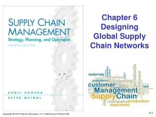
Total Landed Cost Minimum Order Quantity Working Capital Product Returns Hidden Costs Inventory Stock-outs
VIDEO • http://www.youtube.com/watch?v=QlZ6TyUaYpw • Supply chain risk reduction
Discounted Cash Flow Analysis • Supply chain decisions are in place for a long time, so they should be evaluated as a sequence of cash flows over that period • Discounted cash flow (DCF) analysis evaluates the present value of any stream of future cash flows and allows managers to compare different cash flow streams in terms of their financial value • Based on the time value of money – a dollar today is worth more than a dollar tomorrow
Discounted Cash Flow Analysis • Compare NPV of different supply chain design options • The option with the highest NPV will provide the greatest financial return
NPV Example: Trips Logistics • How much space to lease in the next three years • Demand = 100,000 units • Requires 1,000 sq. ft. of space for every 1,000 units of demand • Revenue = $1.22 per unit of demand • Decision is whether to sign a three-year lease or obtain warehousing space on the spot market • Three-year lease: cost = $1 per sq. ft. • Spot market: cost = $1.20 per sq. ft. • k = 0.1
NPV Example: Trips Logistics C0 = 1.22 * 100,000 = $122,000 C1 = (1.22 * 100,000) * (1/ (1+.1))1 = $110,909 C2 = (1.22 * 100,000) * (1/ (1+.1))2 = $100,826 Total Income = $333,735
NPV Example: Trips Logistics • How much space to lease in the next three years • Demand = 100,000 units • Requires 1,000 sq. ft. of space for every 1,000 units of demand • Revenue = $1.22 per unit of demand • Decision is whether to sign a three-year lease or obtain warehousing space on the spot market • Three-year lease: cost = $1 per sq. ft. • Spot market: cost = $1.20 per sq. ft. • k = 0.1
NPV Example: Trips Logistics C0 = 1 * 100,000 = $100,000 C1 = (1 * 100,000) * (1/ (1+.1))1 = $90,909 C2 = (1 * 100,000) * (1/ (1+.1))2 = $82,644 Total Costs (three year lease) = $273,553 Total Income = $333,735 Total Profit = $60,181
NPV Example: Trips Logistics • How much space to lease in the next three years • Demand = 100,000 units • Requires 1,000 sq. ft. of space for every 1,000 units of demand • Revenue = $1.22 per unit of demand • Decision is whether to sign a three-year lease or obtain warehousing space on the spot market • Three-year lease: cost = $1 per sq. ft. • Spot market: cost = $1.20 per sq. ft. • k = 0.1
NPV Example: Trips Logistics C0 = 1 * 100,000 = $120,000 C1 = (1 * 100,000) * (1/ (1+.1))1 = $109,090 C2 = (1 * 100,000) * (1/ (1+.1))2 = $99,173 Total Costs (no lease) = $328,264 Total Income = $333,735 Total Profit = $5,471
Representations of Uncertainty • Binomial Representation of Uncertainty • Other Representations of Uncertainty
Binomial Representationsof Uncertainty • When moving from one period to the next, the value of the underlying factor (e.g., demand or price) has only two possible outcomes – up or down • The underlying factor moves up by a factor or u > 1 with probability p, or down by a factor d < 1 with probability 1-p • Assuming a price P in period 0, for the multiplicative binomial, the possible outcomes for the next four periods: • Period 1: Pu, Pd • Period 2: Pu2, Pud, Pd2 • Period 3: Pu3, Pu2d, Pud2, Pd3 • Period 4: Pu4, Pu3d, Pu2d2, Pud3, Pd4
Binomial Representationsof Uncertainty • When moving from one period to the next, the value of the underlying factor (e.g., demand or price) has only two possible outcomes – up or down • The underlying factor moves up by a factor or u > 1 with probability p, or down by a factor d < 1 with probability 1-p • Assuming a price P in period 0, for the multiplicative binomial, the possible outcomes for the next four periods: • Period 1: Pu, Pd • Period 2: Pu2, Pud, Pd2 • Period 3: Pu3, Pu2d, Pud2, Pd3 • Period 4: Pu4, Pu3d, Pu2d2, Pud3, Pd4
Door 1 $100 2
Door 1 $100*2= $200 2
Door 1 $100/2= $100 2
Door 1 $100/2= $50 2
Door 1 $50/2= $25 2
Binomial Representationsof Uncertainty • When moving from one period to the next, the value of the underlying factor (e.g., demand or price) has only two possible outcomes – up or down • The underlying factor moves up by a factor or u > 1 with probability p, or down by a factor d < 1 with probability 1-p • Assuming a price P in period 0, for the multiplicative binomial, the possible outcomes for the next four periods: • Period 1: Pu, Pd • Period 2: Pu2, Pud, Pd2 • Period 3: Pu3, Pu2d, Pud2, Pd3 • Period 4: Pu4, Pu3d, Pu2d2, Pud3, Pd4
Binomial Representationsof Uncertainty • In general, for multiplicative binomial, period T has all possible outcomes Putd(T-t), for t = 0,1,…,T • From state Puad(T-a) in period t, the price may move in period t+1 to either • Pua+1d(T-a) with probability p, or • Puad(T-a)+1 with probability (1-p)
Binomial Representationsof Uncertainty • For the additive binomial, the states in the following periods are: • Period 1: P+u, P-d • Period 2: P+2u, P+u-d, P-2d • Period 3: P+3u, P+2u-d, P+u-2d, P-3d • Period 4: P+4u, P+3u-d, P+2u-2d, P+u-3d, P-4d • In general, for the additive binomial, period T has all possible outcomes P+tu-(T-t)d, for t=0, 1, …, T
Evaluating Network Design Decisions Using Decision Trees • A manager must make many different decisions when designing a supply chain network • Many of them involve a choice between a long-term (or less flexible) option and a short-term (or more flexible) option • If uncertainty is ignored, the long-term option will almost always be selected because it is typically cheaper • Such a decision can eventually hurt the firm, however, because actual future prices or demand may be different from what was forecasted at the time of the decision • A decision tree is a graphic device that can be used to evaluate decisions under uncertainty
Decision Tree Methodology • Identify the duration of each period (month, quarter, etc.) and the number of periods T over the which the decision is to be evaluated. • Identify factors such as demand, price, and exchange rate, whose fluctuation will be considered over the next T periods. • Identify representations of uncertainty for each factor; that is, determine what distribution to use to model the uncertainty. • Identify the periodic discount rate k for each period. • Represent the decision tree with defined states in each period, as well as the transition probabilities between states in successive periods. • Starting at period T, work back to period 0, identifying the optimal decision and the expected cash flows at each step. Expected cash flows at each state in a given period should be discounted back when included in the previous period.
Decision Tree Methodology:Trips Logistics • Decide whether to lease warehouse space for the coming three years and the quantity to lease • Long-term lease is currently cheaper than the spot market rate • The manager anticipates uncertainty in demand and spot prices over the next three years • Long-term lease is cheaper but could go unused if demand is lower than forecast; future spot market rates could also decrease • Spot market rates are currently high, and the spot market would cost a lot if future demand is higher than expected
Trips Logistics: Three Options • Get all warehousing space from the spot market as needed • Sign a three-year lease for a fixed amount of warehouse space and get additional requirements from the spot market • Sign a flexible lease with a minimum change that allows variable usage of warehouse space up to a limit with additional requirement from the spot market
Trips Logistics • 1000 sq. ft. of warehouse space needed for 1000 units of demand • Current demand = 100,000 units per year • Binomial uncertainty: Demand can go up by 20% with p = 0.5 or down by 20% with 1-p = 0.5 • Lease price = $1.00 per sq. ft. per year • Spot market price = $1.20 per sq. ft. per year • Spot prices can go up by 10% with p = 0.5 or down by 10% with 1-p = 0.5 • Revenue = $1.22 per unit of demand • k = 0.1
Trips Logistics Decision Tree (Fig. 6.2) Period 2 Period 1 D=144 Period 0 p=$1.45 0.25 D=144 0.25 p=$1.19 D=120 0.25 p=$1.32 D=96 0.25 p=$1.45 0.25 D=144 0.25 D=120 p=$0.97 p=$1. 08 D=100 D=96 0.25 p=$1.20 p=$1.19 D=80 D=96 p=$1.32 p=$0.97 0.25 D=64 p=$1.45 D=80 p=$1.08 D=64 p=$1.19 D=64 p=$0.97
Trips Logistics Example • Analyze the option of not signing a lease and obtaining all warehouse space from the spot market • Start with Period 2 and calculate the profit at each node • For D=144, p=$1.45, in Period 2: C(D=144, p=1.45,2) = 144,000x1.45 = $208,800 P(D=144, p =1.45,2) = 144,000x1.22 – C(D=144,p=1.45,2) = 175,680-208,800 = -$33,120 • Profit at other nodes is shown in Table 6.1
Trips Logistics Decision Tree (Fig. 6.2) Period 2 Period 1 D=144 Period 0 p=$1.45 0.25 D=144 0.25 p=$1.19 D=120 0.25 p=$1.32 D=96 0.25 p=$1.45 0.25 D=144 0.25 D=120 p=$0.97 p=$1. 08 D=100 D=96 0.25 p=$1.20 p=$1.19 D=80 D=96 p=$1.32 p=$0.97 0.25 D=64 p=$1.45 D=80 p=$1.08 D=64 p=$1.19 D=64 p=$0.97
Trips Logistics Example • Expected profit at each node in Period 1 is the profit during Period 1 plus the present value of the expected profit in Period 2 • Expected profit EP(D=, p=,1) at a node is the expected profit over all four nodes in Period 2 that may result from this node • PVEP(D=,p=,1) is the present value of this expected profit and P(D=,p=,1), and the total expected profit, is the sum of the profit in Period 1 and the present value of the expected profit in Period 2
Trips Logistics Decision Tree (Fig. 6.2) Period 2 Period 1 D=144 Period 0 p=$1.45 0.25 D=144 0.25 p=$1.19 D=120 0.25 p=$1.32 D=96 0.25 p=$1.45 0.25 D=144 0.25 D=120 p=$0.97 p=$1. 08 D=100 D=96 0.25 p=$1.20 p=$1.19 D=80 D=96 p=$1.32 p=$0.97 0.25 D=64 p=$1.45 D=80 p=$1.08 D=64 p=$1.19 D=64 p=$0.97
Trips Logistics Example • From node D=120, p=$1.32 in Period 1, there are four possible states in Period 2 • Evaluate the expected profit in Period 2 over all four states possible from node D=120, p=$1.32 in Period 1 to be EP(D=120,p=1.32,1) = 0.25xP(D=144,p=1.45,2) + 0.25xP(D=144,p=1.19,2) + 0.25xP(D=96,p=1.45,2) + 0.25xP(D=96,p=1.19,2) = 0.25x(-33,120)+0.25x4,320+0.25x(-22,080)+0.25x2,880 = -$12,000
Trips Logistics Decision Tree (Fig. 6.2) Period 2 Period 1 D=144 Period 0 p=$1.45 0.25 D=144 0.25 p=$1.19 D=120 0.25 p=$1.32 D=96 0.25 p=$1.45 0.25 D=144 0.25 D=120 p=$0.97 p=$1. 08 D=100 D=96 0.25 p=$1.20 p=$1.19 D=80 D=96 p=$1.32 p=$0.97 0.25 D=64 p=$1.45 D=80 p=$1.08 D=64 p=$1.19 D=64 p=$0.97
Trips Logistics Decision Tree (Fig. 6.2) Period 2 Period 1 D=144 Period 0 p=$1.45 0.25 D=144 0.25 p=$1.19 D=120 0.25 p=$1.32 D=96 0.25 p=$1.45 0.25 D=144 0.25 D=120 p=$0.97 p=$1. 08 D=100 D=96 0.25 p=$1.20 p=$1.19 D=80 D=96 p=$1.32 p=$0.97 0.25 D=64 p=$1.45 D=80 p=$1.08 D=64 p=$1.19 D=64 p=$0.97
Trips Logistics Example • From node D=120, p=$1.08 in Period 1, there are four possible states in Period 2 • Evaluate the expected profit in Period 2 over all four states possible from node D=120, p=$1.08 in Period 1 to be EP(D=120,p=1.32,1) = 0.25xP(D=144,p=1.19,2) + 0.25xP(D=144,p=0.97,2) + 0.25xP(D=96,p=1.19,2) + 0.25xP(D=96,p=0.97,2) = 0.25x4,320+0.25x36,000+0.25x2,880+0.25x24,000 = $16,800