Advances in Time-Dependent Density Matrix Renormalization Group Techniques
This article explores the latest advancements in time-dependent density matrix renormalization group (t-DMRG) methods as developed by Adrian Feiguin and collaborators. It summarizes key literature on ground state predictions, wave-function transformations, and the application of Suzuki-Trotter expansions for time evolution in quantum many-body systems. We discuss techniques to efficiently handle real-time dynamics, including error minimization and adaptive basis tracking, highlighting significant contributions from various authors in the field, thereby guiding future research in quantum simulation and transport phenomena.

Advances in Time-Dependent Density Matrix Renormalization Group Techniques
E N D
Presentation Transcript
The time-dependent Adrian Feiguin
Some literature • G. Vidal, PRL 93, 040502 (2004) • S.R.White and AEF, PRL 93, 076401 (2004) • Daley et al, J. Stat. Mech.: Theor. Exp. P04005 (2004) • AEF and S.R.White, PRB 020404 (2005) • U. Schollwoeck and S.R. White, arXiv:cond-mat/0606018
Ground state prediction When we add a site to the left block we represent the new basis states as: Similarly for the right block:
The wave-function transformation Before the transformation, the superblock state is written as: After the transformation, we add a site to the left block, and we “spit out” one from the right block After some algebra, and assuming , one readily obtains:
Solving the t-d Schrödinger Equation Let us assume we know the eigenstates of H In reality, we work in some arbitrary basis Mixture of excited states with oscillating terms with different frequencies Typically we avoid high freq. oscillations by adding a phase
Time evolution and DMRG: First attempts • Cazalilla and Marston, PRL 88, 256403 (2002). Use the infinite system method to find the ground state, and evolved in time using this fixed basis without sweeps. This is not quasiexact. However, they found that works well for transport in chains for short to moderate time intervals. t=0 t= τ t=2τ t=3τ t=4τ • Luo, Xiang and Wang, PRL 91, 049901 (2003) showed how to target correctly for real-time dynamics. They target ψ(t=0), ψ(t= τ) , ψ(t=2τ) , ψ(t=3τ)… t=0 t= τ t=2τ t=3τ t=4τ This is quasiexact as τ→0if you add sweeping. The problem with this idea is that you keep track of all the history of the time-evolution, requiring large number of states m. It becomes highly inefficient.
... In a truncated basis: t=0 Hilbert space Adaptive Time-dependent DMRG: We need to “follow” the state in the Hilbert space adapting the basis at every step t=4 τ t=3 τ t=5τ t=2 τ t= τ S.R.White and AEF, PRL (2004), Daley et al, J. Stat. Mech.: Theor. Exp. (2004);AEF and S.R.White, PRB (2005), Rapid Comm. Based on TEBD ideas by G. Vidal, PRL (94).
... H= H1 + H2 + H3 + H4 + H5 + H6 Evolution operator We would feel tempted to do something like: But it turns out that because This actually would give you an error of the order of t2, similar to a 1st order S-T expansion…
Suzuki-Trotter approach ... H= H1 + H2 + H3 + H4 + H5 + H6 HA= H2 + H4 + H6 HB= H1 + H3 + H5
Suzuki-Trotter expansions We want to write with We want to choose the a’s and b’s such that they kill the first K coefficients CK, minimizing the number of factors P for a given order, to obtain We will impose the conditions that the operators enter symmetrically in the decomposition and I.P Omelyan et al., Comp. Phys. Commmun. 146, 188 (2002) and references therein.
Suzuki-Trotter expansions First order: Second order: We kill the second order term by choosing a=1/2; b=1
Suzuki-Trotter expansions Fourth order: One solution (the most convenient expression) has the form (Forest-Ruth formula) with
1st order Suzuki-Trotter decomposition: So the time-evolution operator is a product of individual link terms. Each link term only involves two-sites interactions => small matrix, easy to calculate! ... Evolution using Suzuki-Trotter No error introduced!
The two-site evolution operatorExample: Heisenberg model (spins) The two-site basis is given by the states |ss’ ={|↑↑;|↑↓;|↓↑; |↓↓} We can easily calculate the Hamiltonian matrix: Exercise:Exponentiate (by hand) the matrix by following these steps: Diagonalize the matrix and calculate eigenvalues and eigenvectors Calculate the exponential of H in the diagonal basis Rotate back to the original basis
Evolving the wave-function e-iτHij We want to apply the evolution operator between the two central sites: As we've seen before, the link evolution operator can be written as And the wave function after the transformation:
` ` ` ` e-iτHij ` tDMRG: The algorithmS.R.White and A.E. Feiguin, PRL (2004), Daley et al, J. Stat. Mech.: Theor. Exp. (2004) We turn off the diagonalization and start applying the evolution operator We start with the finite system algorithm to obtain the ground state We move to the end to start time-evolution
` ` ` ` ` ` ` ` e-iτHij e-iτHij e-iτHij e-iτHij e-iτHij tDMRG: The algorithm S.R.White and A.E. Feiguin, PRL (2004), Daley et al, J. Stat. Mech.: Theor. Exp. (2004) Depending on the S-T break-up, a few sweeps evolve a time step Each link term only involves two-sites interactions: small matrix, easy to calculate! Much faster than Lanczos!
Time-step targeting method What if we don’t have a “nice” Hamiltonian, and S-T cannot be applied The time-evolution can be implemented in various ways: 1) Krylov basis: Calculate Lanczos (tri-diagonal) matrix, and exponentiate. (time consuming) 2) Runge-Kutta. (non-unitary!) • We target one time step accurately, then we move to the next step. • We keep track of intermediate points between t and t+τ t=4τ t=0 t=τ t=2τ t=3τ AEF and S. R.White, PRB (05). See also P. Schmitteckert, PRB 70, 121302(2004)
Sources of error • Suzuki-Trotter error: Can be controlled by using higher order expansions, or smaller time-steps • Truncation error: In principle it can be controlled by keeping more DMRG states as the entanglement grows. Caveat: only works for “well-behaved” problems, since typically the entanglement grows uncontrollably. • Runge-Kutta/Krylov: the error is dominated by the truncation error. Recipe: instead of fixing the number of states for the simulation, we fix the truncation error, and we let the algorithm determine the optimal number of states… until the basis grows too large and the simulation breaks down. Hopefully this will enable us to go to large times…
S=1 Heisenberg chain (L=32; t=8) time targeting +RK 1st order S-T 4th order S-T
For smaller time-step we need more iterations accumulation of error
Comparing S-T and time step targeting • S-T is fast and efficient for one-dimensional geometries with nearest neighbor interactions • S-T error depends strongly on the Trotter error but it can be reduced by using higher order expansions. • Time step targeting (Krylov,RK) can be applied to ladders and systems with long range interactions • It has no Trotter error, you can use a larger time-step, but it is more time consuming and you need more DMRG states. • In RK simulations it is a good practice to do an intermediate sweep without evolving in time to improve the basis. • Time evolution using RK is non-unitary (dangerous!). Krylov expansion is the right choice.
Applications • Transport in nano-structures • Spectral properties, optical conductivity… • Systems driven out of equilibrium, quenches. • Time-dependent Hamiltonians. • Decoherence: Free induction decay, Hahn echo, Rabi oscillations, pulse sequences… …
The enemy: Entanglement growth We have seen that the truncation error, or the number of state that we need to keep to control it, depends fundamentally on the entanglement • We need to understand this behavior if we want to learn how to fight it! • Possible scenarios: • Global quench • Local quench • Periodic quench • Adiabatic quench • … All of a sudden, we are no longer in the ground-state, but some high energy state. Important questions: thermalization vs. integrability
E-growth: global quench Calabrese and Cardy, JStatM (05)
Global quench: qualitative picture Region A (lengh l) B time B 2vt 2vt t t=0 2vt<l We assume that entangled pairs of quasi-particles are created at t=0, and they propagate with maximum velocity Calabrese and Cardy, JStatM (05)
Global quench: qualitative picture Region A (lengh l) B time B t t=0 2vt>l The number of entangled pairs saturates Calabrese and Cardy, JStatM (05)
Local quench: qualitative picture Region A Region B l’=vt time t t=0 The perturbation propagates from the center, splitting the system into two pieces, inside and outside of the light-cone Calabrese and Cardy, JStatM (07)
Computational cost Global quench: Local quench: Adiabatic quench: