Download
1 / 64
650 likes | 918 Views
National Central University @ Jhong-Li, Taiwan November 20, 2012.

E N D
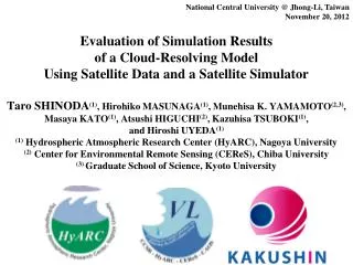
National Central University @ Jhong-Li, Taiwan November 20, 2012 Evaluation of Simulation Results of a Cloud-Resolving ModelUsing Satellite Data and a Satellite SimulatorTaro SHINODA(1), Hirohiko MASUNAGA(1), Munehisa K. YAMAMOTO(2,3), Masaya KATO(1), Atsushi HIGUCHI(2), Kazuhisa TSUBOKI(1), and Hiroshi UYEDA(1)(1) Hydrospheric Atmospheric Research Center (HyARC), Nagoya University(2) Center for Environmental Remote Sensing (CEReS), Chiba University(3) Graduate School of Science, Kyoto University
National Central University @ Jhong-Li, Taiwan November 20, 2012 Introduction of Meteorological Laboratory, HyARC, Nagoya UniversityTaro Shinoda (Hydrospheric Atmospheric Research Center, Nagoya University)
Hiroshi Uyeda, Professor. Kazuhisa Tsuboki, Professor. Taro Shinoda, Assistant professor. Tadayasu Ohigashi, Assistant Professor Our research field is extreme mesoscale phenomena; such as typhoon, heavy rainfall/snowfall, gust wind/tornado using two X-band polarimetric Doppler radars and a cloud resolving model (CReSS). Laboratory of Meteorology, HyARC, Nagoya University X-band polarimetric Doppler radars Typhoon T0418 simulated by CReSS
Gin(Silver) Kin(Gold) @Gifu Univ. @HyARC HyARC polarimetric Doppler radars The HyARC X-band polarimetric Doppler radars were installed in November 2007.
Conventional Radar vs. Polarimetric Radar Only horizontal polarization Conventional radar Vertical polarization Horizontal polarization Polarization radar ・Transmit horizontal and vertical polarizations as same power and phase.
Polarimetric Parameters Obtained parameters * Radar reflectivity (Zh) * Doppler velocity (V) * Differential reflectivity (Zdr) * Correlation coefficient between horizontal and vertical polarization signals(ρhv) * Differential propagation phase (Φdp) * Specific differential phase (KDP) For horizontal polarization ・ Signal: large ・ Phase delay: large For vertical polarization ・ Signal: small ・ Phase delay: small Vertical polarization Horizontal polarization Polarization radar ・Transmit horizontal and vertical polarizations as same power and phase.
Shape of precipitation particlesvs polarimetric parameter (Zdr) Snowflakes: 0 ~ 0.5 dB Graupels: -0.5 ~ 0 dB (Vertical axis longer) Hailstones: 0 dB (Almost shpere) Houze (1993) Raindrops: 0 ~ 5.0 dB Horizontal scattered section is larger for the larger raindrops → positive Zdr
A sample of particle identification (Aug. 28, 2008) Shinoda et al. MWR submitted ・Particle identification was examined using Zh, Zdr, ρhv, KDP, and T. ・Large raindrops (D0 ~ 2.5 mm) exist below the ML. ・Dry and wet graupels (orange/red colors) exist around the ML. → The melting of graupels should form large raindrops below the ML and caused a large amount of rainfall.
Particle identificationin comparison with CReSS simulation NW SE ・ A large amount of graupel (blue contours) exists above the ML. ・ These grauples fall with melting and form a large amount of large raindrops. ・As a large amount of cloud water intrudes (red contours), graupels should be formed by a riming process. Shinoda et al. MWR submitted
Toward the confirmation of particle identification: HYVIS Obs. The hydrometeor videosonde (HYVIS) ・ In situ observation system to obtain images of cloud particles: such as phase, size, shape, and number concentration. ・ We conducted simultaneous observation using both the HYVIS and polarimetric radar in 2008, 2010, 2011, and 2012 (this year).
Toward the confirmation of particle identification: HYVIS Obs. The hydrometeor videosonde (HYVIS) ・ In situ observation system to obtain images of cloud particles: such as phase, size, shape, and number concentration. ・ We conducted simultaneous observation using both the HYVIS and polarimetric radar in 2008, 2010, 2011, and 2012 (this year).
Sample of a HYVIS observation Zh 24.8 dBZe 0.08 dB Column type ice crystals were observed at 5800 m (-5℃) positive X: HYVIS 0.5mm ρhv Kdp 0.41º/km 0.996 Zdr positive 2mm
A plan of our field experiment in Palau (in 2013 and 2014) Typhoon Pressure drop and enhancementof vorticity Aimeliik Observation May & June 2013 December 2013 May & June 2014 Vortex: D ~100 ㎞ Vortex: D ~10 km Vortex: D = 300 ~ 500 ㎞ From Houze (2010) HYVIS Observation N 60 km N The Philippines Ngarchelong Aimeliik 80 km Palau VHT Palau 60 km E E Courtesy of Prof. Uyeda
Our own cloud-resolving model (CReSS) ・ CReSS develop from 1997 by Prof. Tsuboki and Mr. Sakakibara. ・ CReSS has non-hydrostatic, compressible equation system and terrain-following coordinate system. ・ CReSS has a bulk cold rain scheme (Qv, Qc, Qr, Qi, Qs, Qg). ・ CReSS is optimized for parallel computers. ・ The basic framework of CReSS resembles the ARPS model.
Niigata heavy rainfall case: July 28-30, 2011 22 JST July 29 01 JST July 30 09 JST July 30 06 JST July 30
Niigata heavy rainfall case: Total rainfall amount (Obs. vs Sim.)
Typhoon Morakot (T0908) simulation: 2.5-km horizontal resolution ・ We have simulated Typhoon Morakot (T0908) using the CReSS to test the framework of the daily simulation for the SoWMEX2010.
Typhoon Morakot (T0908) simulation: 2.5-km horizontal resolution ・ Maximum accumulated rainfall amount during this simulation reaches over 4300 mm around the CMR over Taiwan Island.
Gifu heavy rainfall case: July 15, 2010 (JMA radar vs CReSS) Observation (JMA-Radar) CReSS Maximum rainfall 350 mm / 6 h No significant rainfall region!
Effect of the simple Data Assimilation Run CReSS: Radar data nudging (Qr and Qv) Observation (JMA-Radar) Maximum rainfall 350 mm / 6 h Heavy rainfall area is reproduced well by radar data nudging!
A regional atmosphere-ocean coupled model (CReSS-NHOES) CReSS NHOES Wave ・NHOES: NonHydrostatic Ocean model for Earth Simulator ・ NHOES is developed by Dr. Aiki of JAMSTEC. ・ We have started to develop of CReSS-NHOEScoupling since 2010 and to conduct daily forecasting from last June. Surface roughness Skin stress + Wave stress U10 Heat & Water fluxes Ufric SST Surface Current Skin stress + Dissipation stress
SST difference with or without 3D ocean coupled model Coupled Sim. – Uncoupled Sim. at 54 hours ・ Large SST difference (> 1℃) appear between 1D and 3D ocean coupled result along the typhoon track and along the warm/cold currents region.
SST difference with or without 3D ocean coupled model Coupled Sim. – Uncoupled Sim. at 54 hours A: EPT (color) across wind (coutor) O: Temperature difference from initial condition(color) ・ Sea temperature above a depth of 30 m (around the bottom of mixed layer: 50 m) decrease (increase) by vertical mixing induced by high wind of the typhoon.
雷雲の電気的半生のモデル化 Modeling of a lightning process in thunderclouds Separation of updraft, gravity (by density of particle) (1) (2) (3) (1) → • Accumulation of electric charge • by hydrometeor particle charging. • (2) Extension of lightning channels. • (3) Charge neutralization. • Lightning process was followed • by MacGoman et al. (2001).
Modeling of a lightning process in thunderclouds Reproduction of thunderclouds Separation of updraft, gravity (by density of particle) (1) (2) (3) (1) → • Accumulation of electric charge • by hydrometeor particle charging. • (2) Extension of lightning channels. • (3) Charge neutralization. • Lightning process was followed • by MacGoman et al. (2001). Reproduction of thunderclouds
Modeling of a lightning process in thunderclouds Reproduction of thunderclouds Reproduction of charge distributions Separation of updraft, gravity (by density of particle) (1) (2) (3) (1) → • Accumulation of electric charge • by hydrometeor particle charging. • (2) Extension of lightning channels. • (3) Charge neutralization. • Lightning process was followed • by MacGoman et al. (2001). Reproduction of charge distributions Reproduction of thunderclouds
Modeling of a lightning process in thunderclouds Reproduction of thunderclouds Reproduction of charge distributions Separation of updraft, gravity (by density of particle) (1) (2) (3) Reproduction of Lightning (1) → • Accumulation of electric charge • by hydrometeor particle charging. • (2) Extension of lightning channels. • (3) Charge neutralization. • Lightning process was followed • by MacGoman et al. (2001). Reproduction of Lightning Reproduction of charge distributions Reproduction of thunderclouds
Lightning simulation result in comparison with the LLS observation Simulated CG Lightning Total: 10644 Positive polarity: 3522 Negative polarity: 7122
Lightning simulation result in comparison with the LLS observation Simulated CG Lightning Total: 10644 Positive polarity: 3522 Negative polarity: 7122 Observed CG Lightning Total: 2588 Positivepolarity: 651 Negative polarity: 1937
National Central University @ Jhong-Li, Taiwan November 20, 2012 Evaluation of Simulation Results of a Cloud-Resolving ModelUsing Satellite Data and a Satellite SimulatorTaro SHINODA(1), Hirohiko MASUNAGA(1), Munehisa K. YAMAMOTO(2,3), Masaya KATO(1), Atsushi HIGUCHI(2), Kazuhisa TSUBOKI(1), and Hiroshi UYEDA(1)(1) Hydrospheric Atmospheric Research Center (HyARC), Nagoya University(2) Center for Environmental Remote Sensing (CEReS), Chiba University(3) Graduate School of Science, Kyoto University
Cloud Resolving Models (CRMs) ・ Cloud Resolving Models (CRMs) explicitly resolve convective clouds, so they are useful tools to analyze the structure of precipitation systems. ・ We have a CRM named Cloud Resolving Storm Simulator (CReSS). ・ CRMs have many uncertainties in cloud microphysical processes. ・ To confirm the accuracy of CRMs, it is useful to compare the results of simulations with those of satellite observations.
Evaluation of CRM simulations using satellite data Masunaga et al. (2010, BAMS) ・ The physical parameters simulated by the CRM were compared with those retrieved by satellite observations. ・The retrieved physical parameters could contain their own biases due to uncertainties in the inversion algorithms. → It is difficult to make an evaluation of the CRM using satellite-derived physical parameters.
A satellite simulator Radiative transfer calculations Masunaga et al. (2010, BAMS) ・ Several satellite simulators are developed in recent several years. ・ It estimates satellite-consistent radiances from the CRM outputs using radiative transfer calculations (forward model). ・ Direct satellite measurements (radiances) should have less uncertainties than retrieved physical parameters.
Satellite Data Simulator Unit (SDSU) ・ SDSU is developed to compute synthetic satellite data from CRM output by Dr. Masunaga. ・ SDSU is designed to simulate * thermal infrared brightness temperature, * microwave brightness temperature, * radar reflectivity, * visible and near-infrared radiances. ・ Input parameters * P, PT, Qv, Qc, Qr, Qi, Qs, Qg, Ni, Ns, Ng, z * SST, Surface winds http://precip.hyarc.nagoya-u.ac.jp/sdsu/sdsu-main.html
TBB-IR distributions (MTSAT vs CReSS-SDSU: May 29, 2010) ・ MTSAT obs.: Well-developed MCSs develop over southeast and southwest far from Taiwan Island. ・ The location and minimum TBB of the southeastern MCS are well reproduced in CReSS-SDSU. ・ The cloud cover is seen over the almost all of the simulation region in the MTSAT obs. and CReSS-SDSU.
Time series of cloud fraction (MTSAT vs CReSS-SDSU)in 2010 June 04 May 15 20 25 30 09 14 19 24 29 ・ The variation of the cloud fraction (CF) is well reproduced. ・ Difference of CF is small (~ 10%), sometimes over 30%. ※ Definition of the cloud column: The column whose difference in temperature between the SST and IR TBB is greater than 15 K.
TBB-IR distributions (MTSAT vs CReSS-SDSU: June 4, 2008) ・ MTSAT obs.: MCSs develop along the Meiyu/Baiu front from southwest of Taiwan to south of Okinawa. ・ Low TBB area expands broadly over the north of the Meiyu/Baiu front in CReSS-SDSU. ・ At this time, the cloud cover in CReSS-SDSU is close to that in the MTSAT observation.
Time series of cloud fraction (MTSAT vs CReSS-SDSU) ): in 2008 20 25 30 June 04 09 14 19 24 May 15 ・ In 2008, the simulated cloud fraction (CF) is larger than the observed one, thus is not reproduced.
Compared PDF/CPDF of TBB-IR (MTSAT vs CReSS-SDSU) in 2010 ・Frequency of UC (TBB < 240 K) of the CReSS-SDSU is larger. ・Frequency of MC/LC (TBB > 250 K) of the CReSS-SDSU is lesser.
Compared PDF/CPDF of TBB-IR (MTSAT vs CReSS-SDSU): in 2008 ・ The shape of the cumulative PDF in 2008 is quite same that in 2010. * Frequency of UC (MC/LC) of the CReSS-SDSU is larger (lesser). ・ However, the difference of the frequency of UC in 2010 is reduced a little that in 2008. ・This should be attributed to the inclusion of cloud ice sedimentation.
TBB-MW 89GHz distributions (AMSR-E vs CReSS-SDSU) ・This frequency is sensitive to ice particles in the upper troposphere. ・If large amount of ice particle exists, TBB shows small values. ・Low TBB areas are seen in the southeast and southwest MCSs. ・Minimum TBB in the simulation is quite lower. → This suggests the excessive existence of solid hydrometeors. ・The area of moderate TBB in the simulation is quite smaller. → The extension of dense stratiform region cannot be reproduced.
Reflectivity distributions(TRMM-PR vs CReSS-SDSU) Height:2 km
Comparison of CFAD(TRMM-PR vs CReSS-SDSU) ・ Distributions of reflectivity below the melting level is reproduced very well in the simulation. ・ Large reflectivity above the melting level should be simulated by the excessive existence of graupels.
Comparison of PDF of reflectivity(TRMM-PR vs CReSS-SDSU) ・ Above the ML(7 km): Frequency (> 24 dBZ) is large quite large in the simulation. → Excessive existence of hydrometeors in the narrow area (convective core). ・ Around the ML(5 km): Frequency (23~25 dBZ) is less in the simulation. → Less extension of stratiform region. ・Below the ML(2 km): Frequency is quite same, but that (> 28 dBZ) is less. → Less extension of stratiform region.