Algorithm Design and Analysis (ADA)
Algorithm Design and Analysis (ADA). 242-535 , Semester 1 2013-2014. Objective introduce DP, its two hallmarks, and two major programming techniques look at two examples: the fibonacci series and LCS. 7. Dynamic Programming. Overview. Dynamic Programming ( DP ) Fibonacci Series

Algorithm Design and Analysis (ADA)
E N D
Presentation Transcript
Algorithm Design and Analysis (ADA) 242-535, Semester 1 2013-2014 • Objective • introduce DP, its two hallmarks, and two major programming techniques • look at two examples: the fibonacci series and LCS 7. Dynamic Programming
Overview • Dynamic Programming (DP) • Fibonacci Series • Features of DP Code • Longest Common Subsequence (LCS) • Towards a Better LCS Algorithm • Recursive Definition of c[] • Is the c[] Algorithm Optimal? • Repeated Subproblems? • LCS() as a DP Problem • Bottom-up Examples • Finding the LCS • Space and Bottom-up
1. Dynamic Programming (DP) • The "programming" in DP predates computing, and means "using tables to store information". • DP is a recursiveprogramming technique: • the problem is recursively described in terms of smilar but smaller subproblems
What makes DP Different? • Optimal solution from optimal parts • An optimal (best) solution to the problem is a composition of optimal (best) subproblem solutions • Repeated (overlapping) sub-problems • the problem contains the same subproblems, repeated many times Hallmark #1 Hallmark #2
Some Famous DP Examples • Unix diff for comparing two files • Smith-Waterman for genetic sequence alignment • determines similar regions between two protein sequences (strings) • Bellman-Ford for shortest path routing in networks • Cocke-Kasami-Younger for parsing context free grammars
2. Fibonacci Series • Series defined by • a0 = 1 • a1 = 1 • an = an-1 + an-2 • Recursive algorithm: • Running Time? O(2n) 1, 1, 2, 3, 5, 8, 13, 21, 34, … fib(n) if n == 0 or n == 1, then return 1 else a = fib(n-1) b= fib(n-2) return a+b
Computing Fibonacci Faster • Fibonacci can be viewed as a DP problem: • the optimal solution (fib(n)) is a combination of optimal sub-solutions (fib(n-1) and fib(n-2)) • There are a lot of repeated subproblems • look at the execution graph (next slide) • 2n subproblems, but only n are different
lots of repeated work, that only gets worse for bigger n • Execution of fib(5):
3. Features of DP Code • Memoization: values returned by recursive calls are stored in a table (array) so they do not need to be recalculated • this can save enormous amount of running time • Bottom-up algorithms: simple solutions are computed first (e.g. fib(0), fib(1), ...), leading to larger solutions (e.g. fib(23), fib(24), ...) • this means that the solutions are added to the table in a fixed order which may allow them to be calculated quicker and the table to be less large
Memoization fib() Algorithm m[] 0 1 • Running time is linear = O(n) • Requires extra space for the m[] table = O(n) fib(n) if(m[n] == 0) then m[n] = fib(n − 1) + fib(n − 2) return m[n] 1 1 2 0 3 0 :: :: 0 n-1
Bottom-up fib() Algorithm int fib(int n) { if (n == 0) return 1; else { int prev = 1; int curr = 1; int temp; for (int i=1; i < n; i++) { temp = prev + curr; prev = curr; curr = temp; } return curr; } } Running time = O(n) Space requirement is 3 variables = O(1) ! this has nothing to do with changing from recursion to a loop, but with changing from top-down to bottom-up execution, which in this case is easier to write as a loop
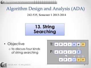
4. Longest Common Subsequence (LCS) • Given two sequences x[1 . . m] and y[1 . . n], find a longest subsequence common to them both. x: A B C B D A B BCBA = LCS(x, y) y: B D C A B A and BDAB BCAB
Brute-force LCS Algorithm Check every subsequence of x[1 . . m] to see if it is also a subsequence of y[1 . . n]. Analysis • Checking time for each subsequence is O(n). • 2msubsequences of x[](can use or not use each element in x). Worst-case running time = O(n*2m),exponential time. SLOW == BAD
5. Towards a Better LCS Algorithm Simplify the problem: • Find the length of a LCS 2. We'll extend the algorithm later to find the LCS.
Prefixes • If X = < A, B, C, B, D, A, B > then • A prefix is x[1 .. 4] == < A, B, C, B > • we abbreviate this as x4 • Also x0 is the empty sequence
Creating a Table of Lengths • c[] is a table (2D array) for storing LCS lengths: c[i, j] = | LCS(x[1. . i], y[1. . j]) | • | s | is the length of a sequence s • Since x is of length m, and y is of length n, then • c[m, n] = | LCS(x, y) |
Calculating LCS Lengths • Since X0 and Y0 are empty strings, their LCS is always empty (i.e. c[0, 0] == 0) • The LCS of an empty string and any other string is empty, so for every i and j: c[0, j] == c[i, 0] == 0
Initial c[] 0 1 2 3 4 5 0 0 0 0 0 0 0 1 0 2 0 3 0 4 0
6. Recursive Definition of c[] • The first line of this definition fills the top row and first column of c[] with 0's, as in the non-recursive approach.
When we calculate c[i, j], there are two cases: • First case:x[i] == y[j]: one more symbol in strings X and Y matches, so the length of LCS Xi and Yjequals the length of LCS of smaller strings Xi-1 and Yi-1 , plus 1
Second case:x[i] != y[j] • As symbols don’t match, our solution is not improved, and the length of LCS(Xi , Yj) is the same as the biggest from before (i.e. max of LCS(Xi, Yj-1) and LCS(Xi-1,Yj)
7. Is c[] Algorithm Optimal? • One advantage of a recursive definition for c[] is that it makes it easy to show that c is optimal by induction • c[i, j] increases the size of a sub-solution (line 2) or uses the bigger of two sub-solutions (line 3) • assuming that a smaller c[] entry is optimal, then a larger c[] entry is optimal. • when combined with the base cases, which are optimal, then c[] is an optimal solution for all entries
Is LCS() Optimal? • c[] is an optimal way to calculate the length of a LCS using smaller optimal solutions (Hallmark #1) • The c[] algorithm can be used to return the LCS (see later), so LCS also has Hallmark #1
LCS Length as Recursive Code LCS(x, y, i, j) ifi == 0 or j == 0 thenc[i, j] ← 0 elseif x[i] == y[ j] then c[i, j] ← LCS(x, y, i–1, j–1) + 1 else c[i, j] ← max(LCS(x, y, i–1, j), LCS(x, y, i, j–1) ) return c[i, j] • The recursive definition of c[] has been changed into a LCS() function which returns c[]
8. Repeated Subproblems? • Does the LCS() algorithm have many repeating (overlapping) subproblems? • i.e. does it have DP Hallmark #2? • Consider the worst case execution • x[i] ≠ y[ j], in which case the algorithm evaluates two subproblems, each with only one parameter decremented
Recursion Tree (in worst cases) Height = m + n. The total work is exponential, but we’re repeating lots of subproblems.
Dynamic Programming Hallmark #2 • The number of distinct LCS subproblems for two strings of lengths m and n is only m*n. • a lot less than 2m+ntotal no. of problems
9. LCS() as a DP Problem • LCS has both DP hallmarks, and so will benefit from the DP programming techniques: • recursion • memoization • bottom-up execution
9.1. Memoization LCS(x, y, i, j) if c[i, j] is empty then // calculate if not already in c[i, j] ifi == 0 or j == 0 thenc[i, j] ← 0 elseif x[i] == y[ j] then c[i, j] ← LCS(x, y, i–1, j–1) + 1 else c[i, j] ← max(LCS(x, y, i–1, j), LCS(x, y, i, j–1) ) return c[i, j] Time = Θ(m*n) == constant work per table entry Space = Θ(m*n)
9.2. Bottom-up Execution • This algorithm works top-down • start with large subsequences, and calculate the smaller subsequences • Let's switch to bottom-up execution • calculate the small subsequences first, then move to larger ones
LCS Length Bottom-up LCS-Length(X, Y) 1. m = length(X) // get the # of symbols in X 2. n = length(Y) // get the # of symbols in Y 3. for i = 1 to m c[i,0] = 0 // special case: Y0 4. for j = 1 to n c[0,j] = 0 // special case: X0 5. for i = 1 to m // for all Xi 6. for j = 1 to n // for all Yj 7. if ( Xi == Yj ) 8. c[i,j] = c[i-1,j-1] + 1 9. else c[i,j] = max( c[i-1,j], c[i,j-1] ) 10. return c the same recursive definition of c[] as before
10. Bottom-up Examples We’ll see how a bottom-up LCS works on: • X = ABCB • Y = BDCAB LCS(X, Y) = BCB X = A BCB Y = B D C A B LCS-length(X, Y) = 3
LCS Example 1 ABCB BDCAB j 0 1 2 3 4 5 i Yj B D C A B Xi 0 A 1 B 2 3 C 4 B X = ABCB; m = |X| = 4 Y = BDCAB; n = |Y| = 5 Allocate array c[5,4]
ABCB BDCAB j 0 1 2 3 4 5 i Yj B D C A B Xi 0 0 0 0 0 0 0 A 1 0 B 2 0 3 C 0 4 B 0 for i = 1 to m c[i,0] = 0 for j = 1 to n c[0,j] = 0
ABCB BDCAB j 0 1 2 3 4 5 i Yj B D C A B Xi 0 0 0 0 0 0 0 A 1 0 0 B 2 0 3 C 0 4 B 0 if ( Xi == Yj ) c[i,j] = c[i-1,j-1] + 1 else c[i,j] = max( c[i-1,j], c[i,j-1] )
ABCB BDCAB j 0 1 2 3 4 5 i Yj B D C A B Xi 0 0 0 0 0 0 0 A 1 0 0 0 0 B 2 0 3 C 0 4 B 0 if ( Xi == Yj ) c[i,j] = c[i-1,j-1] + 1 else c[i,j] = max( c[i-1,j], c[i,j-1] )
ABCB BDCAB j 0 1 2 3 4 5 i Yj B D C A B Xi 0 0 0 0 0 0 0 A 1 0 0 0 0 1 B 2 0 3 C 0 4 B 0 if ( Xi == Yj ) c[i,j] = c[i-1,j-1] + 1 else c[i,j] = max( c[i-1,j], c[i,j-1] )
ABCB BDCAB j 0 1 2 3 4 5 i Yj B D C A B Xi 0 0 0 0 0 0 0 A 1 0 0 0 0 1 1 B 2 0 3 C 0 4 B 0 if ( Xi == Yj ) c[i,j] = c[i-1,j-1] + 1 else c[i,j] = max( c[i-1,j], c[i,j-1] )
ABCB BDCAB j 0 1 2 3 4 5 i Yj B D C A B Xi 0 0 0 0 0 0 0 A 1 0 0 0 0 1 1 B 2 0 1 3 C 0 4 B 0 if ( Xi == Yj ) c[i,j] = c[i-1,j-1] + 1 else c[i,j] = max( c[i-1,j], c[i,j-1] )
ABCB BDCAB j 0 1 2 3 4 5 i Yj B D C A B Xi 0 0 0 0 0 0 0 A 1 0 0 0 0 1 1 B 2 0 1 1 1 1 3 C 0 4 B 0 if ( Xi == Yj ) c[i,j] = c[i-1,j-1] + 1 else c[i,j] = max( c[i-1,j], c[i,j-1] )
ABCB BDCAB j 0 1 2 3 4 5 i Yj B D C A B Xi 0 0 0 0 0 0 0 A 1 0 0 0 0 1 1 B 2 0 1 1 1 1 2 3 C 0 4 B 0 if ( Xi == Yj ) c[i,j] = c[i-1,j-1] + 1 else c[i,j] = max( c[i-1,j], c[i,j-1] )
ABCB BDCAB j 0 1 2 3 4 5 i Yj B D C A B Xi 0 0 0 0 0 0 0 A 1 0 0 0 0 1 1 B 2 0 1 1 1 1 2 3 C 0 1 1 4 B 0 if ( Xi == Yj ) c[i,j] = c[i-1,j-1] + 1 else c[i,j] = max( c[i-1,j], c[i,j-1] )
ABCB BDCAB j 0 1 2 3 4 5 i Yj B D C A B Xi 0 0 0 0 0 0 0 A 1 0 0 0 0 1 1 B 2 0 1 1 1 1 2 3 C 0 1 1 2 4 B 0 if ( Xi == Yj ) c[i,j] = c[i-1,j-1] + 1 else c[i,j] = max( c[i-1,j], c[i,j-1] )
ABCB BDCAB j 0 1 2 3 4 5 i Yj B D C A B Xi 0 0 0 0 0 0 0 A 1 0 0 0 0 1 1 B 2 0 1 1 1 1 2 3 C 0 1 1 2 2 2 4 B 0 if ( Xi == Yj ) c[i,j] = c[i-1,j-1] + 1 else c[i,j] = max( c[i-1,j], c[i,j-1] )
ABCB BDCAB j 0 1 2 3 4 5 i Yj B D C A B Xi 0 0 0 0 0 0 0 A 1 0 0 0 0 1 1 B 2 0 1 1 1 1 2 3 C 0 1 1 2 2 2 4 B 0 1 if ( Xi == Yj ) c[i,j] = c[i-1,j-1] + 1 else c[i,j] = max( c[i-1,j], c[i,j-1] )
ABCB BDCAB j 0 1 2 34 5 i Yj B D C A B Xi 0 0 0 0 0 0 0 A 1 0 0 0 0 1 1 B 2 0 1 1 1 1 2 3 C 0 1 1 2 2 2 4 B 0 1 1 2 2 if ( Xi == Yj ) c[i,j] = c[i-1,j-1] + 1 else c[i,j] = max( c[i-1,j], c[i,j-1] )
ABCB BDCAB j 0 1 2 3 4 5 i Yj B D C A B Xi 0 0 0 0 0 0 0 A 1 0 0 0 0 1 1 B 2 0 1 1 1 1 2 3 C 0 1 1 2 2 2 3 4 B 0 1 1 2 2 if ( Xi == Yj ) c[i,j] = c[i-1,j-1] + 1 else c[i,j] = max( c[i-1,j], c[i,j-1] )
Running Time • The bottom-up LCS algorithm calculates the values of each entry of the array c[m, n] • So what is the running time? O(m*n) • Since each c[i, j] is calculated in constant time, and there are m*n elements in the array
Example 2 n elements in y[1..n] m elements in x[1..m] B == B, somax + 1
11. Finding the LCS • So far, we have found the length of LCS. • We want to modify this algorithm to have it calculate LCS of X and Y Each c[i, j] depends on c[i-1, j] and c[i, j-1] or c[i-1, j-1] For each c[i, j] we can trace back how it was calculated: 2 2 For example, here c[i, j] = c[i-1, j-1] +1 = 2+1=3 2 3