Algorithm Design and Analysis

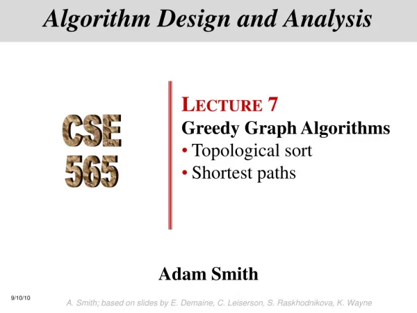
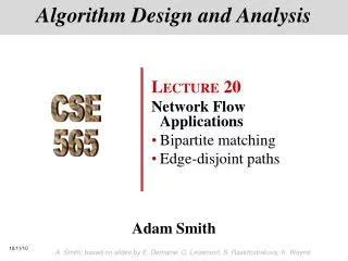
1. LECTURE 21 • Network Flow • Finish bipartite matching • Capacity-scaling algorithm Algorithm Design and Analysis CSE 565 Adam Smith A. Smith; based on slides by E. Demaine, C. Leiserson, S. Raskhodnikova, K. Wayne

2. 1 1' 2 2' 3 3' 4 4' L R 5 5' Marriage Theorem • Marriage Theorem. [Frobenius 1917, Hall 1935] Let G = (L  R, E) be a bipartite graph with |L| = |R|. Then, G has a perfect matching iff • |N(S)|  |S| for all subsets S L. • Pf.  This was the previous observation. No perfect matching: S = { 2, 4, 5 } N(S) = { 2', 5' }.

3. Proof of Marriage Theorem • Pf.  Suppose G does not have a perfect matching. • Formulate as a max flow problem with 1 constraints on edges from L to R and let (A, B) be min cut in G'. • Key property #1 of this graph: min-cut cannot use edges. • So cap(A, B) = |L B | + |R A| • Key property #2: integral flow is still a matching • By max-flow min-cut, cap(A, B) < |L|. • Choose S = L A. • Since min cut can't use  edges: N(S)  R A. • |N(S)| |R A| = cap(A, B) - | L B| < |L| - |L B| = | S|. ▪ 1 G'  1'  A 1 S= {2, 4, 5}L B= {1, 3}R A= {2', 5'}N(S) = {2', 5'} 2'  1 2 s 3' 1 3 4 t 4' 5 1 5'

4. Bipartite Matching: Running Time • Which max flow algorithm to use for bipartite matching? • Generic augmenting path: O(mval(f*)) = O(mn). • Capacity scaling: O(m2log C ) = O(m2). • Shortest augmenting path (not covered in class): O(m n1/2). • Non-bipartite matching. • Structure of non-bipartite graphs is more complicated, butwell-understood. [Tutte-Berge, Edmonds-Galai] • Blossom algorithm: O(n4). [Edmonds 1965] • Best known: O(m n1/2).[Micali-Vazirani1980] • Recently: better algorithms for dense graphs, e.g. O(n2.38) [Harvey, 2006]

5. Exercise • A bipartite graph is k-regular if |L|=|R| and every vertex (regardless of which side it is on) has exactly k neighbors • Prove or disprove: every k-regular bipartite graph has a perfect matching

6. Faster algorithms when capacities are large

7. 1 1 X X 0 1 X X 1 1 X X Ford-Fulkerson: Exponential Number of Augmentations • Q. Is generic Ford-Fulkerson algorithm polynomial in input size? • A. No. If max capacity is C, then algorithm can take C iterations. • Intuition: we’re choosing the wrong paths! m, n, and log C 1 1 1 0 0 0 0 X C C C C 1 1 0 1 0 t t X s s C C C C 1 0 0 0 0 X 2 2

8. Choosing Good Augmenting Paths • Use care when selecting augmenting paths. • Some choices lead to exponential algorithms. • Clever choices lead to polynomial algorithms. • If capacities are irrational, algorithm not guaranteed to terminate! • Goal: choose augmenting paths so that: • Can find augmenting paths efficiently. • Few iterations. • Choose augmenting paths with: [Edmonds-Karp 1972, Dinitz 1970] • Max bottleneck capacity. • Sufficiently large bottleneck capacity. • Fewest number of edges.

9. Capacity Scaling • Intuition. Choosing path with highest bottleneck capacity increases flow by max possible amount. • Don't worry about finding exact highest bottleneck path. • Maintain scaling parameter . • Gf() = subgraphof the residual graph with only arcsofcapacityat least . 4 4 110 102 110 102 1 s s t t 122 170 122 170 2 2 Gf Gf (100)

10. Capacity Scaling Scaling-Max-Flow(G, s, t, c) { foreache E f(e)  0  smallest power of 2 greater than or equal to C Gf residual graph while ( 1) { Gf()-residual graph while (there exists augmenting path P in Gf()) { faugment(f, c, P) // augment flow by  update Gf() }  / 2 } returnf }

11. Capacity Scaling: Correctness • Assumption. All edge capacities are integers between 1 and C. • Integrality invariant. All flow and residual capacity values are integral. • Correctness. If the algorithm terminates, then f is a max flow. • Pf. • By integrality invariant, when  = 1  Gf() = Gf. • Upon termination of  = 1 phase, there are no augmenting paths. ▪

12. Capacity Scaling: Running Time • Lemma 1. The outer while loop repeats 1 + log2 C times. • Pf. Initially C  < 2C.  decreases by a factor of 2 each iteration. ▪ • Lemma 2. Let f be the flow at the end of a -scaling phase. Then the value of the maximum flow f* is at most v(f) + m. (Sanity check: |v(f*) – v(f)| m, and  shrinks, so v(f) converges towards v(f*) ) • Lemma 3. There are at most 2m augmentations per scaling phase. • Let f be the flow at the end of the previous scaling phase. • Lemma 2 v(f*) v(f) + m (2). • Each augmentation in a -phase increases v(f) by at least . ▪ • Theorem. The scaling max-flow algorithm finds a max flow in O(mlog C) augmentations. It can be implemented to run in O(m2log C) time. ▪ proof on next slide (Why?)

13. Capacity Scaling: Running Time • Lemma 2. Let f be the flow at the end of a -scaling phase. Then value of the maximum flow is at most v(f) + m. • Pf. (almost identical to proof of max-flow min-cut theorem) • We show that at the end of a -phase, there exists a cut (A, B) such that cap(A, B) v(f) + m. • Choose A to be the set of nodes reachable from s in Gf(). • By definition of A, s A. • By definition of f, t A. • So v(f*)-v(f) ≤ cap(A,B) – v(f) ≤ m A B t s original network

14. Best Known Algorithms For Max Flow • Reminder: The scaling max-flow algorithm runs in O(m2log C) time. • Currently there are algorithms that run in time • O(mn log n) • O(n3) • O(min(n2/3, m1/2) m log n log C) • Active topic of research: • Flow algorithms for specific types of graphs • Special cases (bipartite matching, etc) • Multi-commodity flow • …

15. What you should know about max flow • How Ford-Fulkerson works • How to use it to find min cuts • How to use it to solve other problems (more examples coming) • max matching • project selection • edge-disjoint paths • vertex-disjoint paths • … • To study: • Review lecture notes/ textbook • Solved exercises in book • Homework problems • Homework exercises • Solve lots of problems!