Download
1 / 38
380 likes | 516 Views
Haplotyping via Perfect Phylogeny. Conceptual Framework and Efficient (almost linear-time) Solutions Dan Gusfield U.C . Davis RECOMB 02, April 2002. Genotypes and Haplotypes. Each individual has two “copies” of each chromosome.

E N D
Haplotyping via Perfect Phylogeny Conceptual Framework and Efficient (almost linear-time) Solutions Dan Gusfield U.C. Davis RECOMB 02, April 2002
Genotypes and Haplotypes Each individual has two “copies” of each chromosome. At each site, each chromosome has one of two alleles (states) denoted by 0 and 1 (motivated by SNPs) 0 1 1 1 0 0 1 1 0 1 1 0 1 0 0 1 0 0 Two haplotypes per individual Merge the haplotypes 2 1 2 1 0 0 1 2 0 Genotype for the individual
Haplotyping Problem • Biological Problem: For disease association studies, haplotype data is more valuable than genotype data, but haplotype data is hard to collect. Genotype data is easy to collect. • Computational Problem: Given a set of n genotypes, determine the original set of n haplotypepairs that generated the n genotypes. This is hopeless without a genetic model.
The Perfect Phylogeny Model We assume that the evolution of extant haplotypes can be displayed on a rooted, directed tree, with the all-0 haplotype at the root, where each site changes from 0 to 1 on exactly one edge, and each extant haplotype is created by accumulating the changes on a path from the root to a leaf, where that haplotype is displayed. In other words, the extant haplotypes evolved along a perfect phylogeny with all-0 root.
The Perfect Phylogeny Model sites 12345 Ancestral haplotype 00000 1 4 Site mutations on edges 3 00010 2 10100 5 10000 01010 01011 Extant haplotypes at the leaves
Justification for Perfect Phylogeny Model • In the absence of recombination each haplotype of any individual has a single parent, so tracing back the history of the haplotypes in a population gives a tree. • Recent strong evidence for long regions of DNA with no recombination. Key to the NIH haplotype mapping project. (See NYT October 30, 2002) • Mutations are rare at selected sites, so are assumed non-recurrent. • Connection with coalescent models.
The Haplotype PhylogenyProblem Given a set of genotypes S, find an explaining set of haplotypes that fits a perfect phylogeny. sites A haplotype pair explains a genotype if the merge of the haplotypes creates the genotype. Example: The merge of 0 1 and 1 0 explains 2 2. S Genotype matrix
The Haplotype PhylogenyProblem Given a set of genotypes, find an explaining set of haplotypes that fits a perfect phylogeny
The Haplotype PhylogenyProblem Given a set of genotypes, find an explaining set of haplotypes that fits a perfect phylogeny 00 1 2 b 00 a a b c c 01 01 10 10 10
The Alternative Explanation No tree possible for this explanation
When does a set of haplotypes to fit a perfect phylogeny? Classic NASC: Arrange the haplotypes in a matrix, two haplotypes for each individual. Then (with no duplicate columns), the haplotypes fit a unique perfect phylogeny if and only if no two columns contain all three pairs: 0,1 and 1,0 and 1,1 This is the 3-Gamete Test
The Alternative Explanation No tree possible for this explanation
The Tree Explanation Again 0 0 1 2 b 0 0 a b a c c 0 1 0 1
Solving the Haplotype Phylogeny Problem (PPH) • Simple Tools based on classical Perfect Phylogeny Problem. • Complex Tools based on Graph Realization Problem (graphic matroid realization).
Simple Tools – treeing the 1’s • For any row i in S, the set of 1 entries in row i specify the exact set of mutations on the path from the root to the least common ancestor of the two leaves labeled i, in every perfect phylogeny for S. • The order of those 1 entries on the path is also the same in every perfect phylogeny for S, and is easy to determine by “leaf counting”.
In any column c, count two for each 1, and count one for each 2. The total is the number of leaves below mutation c, in every perfect phylogeny for S. So if we know the set of mutations on a path from the root, we know their order as well. Leaf Counting S Count 4 4 2 2 1 1 1
The Subtree of 1’s is Forced The columns of S with at least one 1 entry specify a unique upper subtree that must be in every perfect phylogeny for S. 2 1 4 3 S a a b b 4 4 2 2 1 1 1
Corollary: A Useful Sufficient Condition If every column of S has at least one 1, then there is a unique perfect phylogeny for S, if there is any. Build the forced tree based on the 1-entries, then every mutation (site) is in the tree, and any 2-entries dictate where the remaining leaves must be attached to the tree.
What to do when the Corollary does not apply? • Build the forced tree of 1-entries. • 2-entries in columns with 1-entries are done. • Remaining problem: 2-entries in columns without any 1-entries
Uniqueness without 1’s There are 8 haplotype solutions that can explain the data, but only one that fits a perfect phylogeny, i.e. only one solution to the PPH problem.
More Simple Tools • For any row i in S, and any column c, if S(i,c) is 2, then in every perfect phylogeny for S, the path between the two leaves labeled i, must contain the edge with mutation c. Further, every mutation c on the path between the two i leaves must be from such a column c.
From Row Data to Tree Constraints Subtree for row i data sites Root 1 2 3 4 5 6 7 i:0 1 0 2 212 The order is known for the red mutations 2 6 4,5,7 order unknown i i
The Graph Theoretic Problem Given a genotype matrix S with n sites, and a red-blue fork for each row i, create a directed tree T where each integer from 1 to n labels exactly one edge, so that each fork is contained in T. i i
Complex Tool: Graph Realization • Let Rn be the integers 1 to n, and let P be an unordered subset of Rn. P is called a path set. • A tree T with n edges, where each is labeled with a unique integer of Rn, realizes P if there is a contiguous path in T labeled with the integers of P and no others. • Given a family P1, P2, P3…Pk of path sets, tree T realizes the family if it realizes each Pi. • The graph realization problem generalizes the consecutive ones problem, where T is a path.
Graph Realization Example 5 P1: 1, 5, 8 P2: 2, 4 P3: 1, 2, 5, 6 P4: 3, 6, 8 P5: 1, 5, 6, 7 1 8 6 2 4 3 7 Realizing Tree T
Graph Realization Polynomial time (almost linear-time) algorithms exist for the graph realization problem – Whitney, Tutte, Cunningham, Edmonds, Bixby, Wagner, Gavril, Tamari, Fushishige. The algorithms are not simple; no known implementations.
Recognizing graphic Matroids • The graph realization problem is the same problem as determining if a binary matroid is graphic, and the algorithms come from that literature. • The fastest algorithm is due to Bixby and Wagner (Math of OR, ) • Representation methods due to Cunningham et al.
Reducing PPH to graph realization We solve any instance of the PPH problem by creating appropriate path sets, so that a solution to the resulting graph realization problem leads to a solution to the PPH problem instance. The key issue: How to encode a fork by path sets.
From Row Data to Tree Constraints Subtree for row i data sites Root 1 2 3 4 5 6 7 i:0 1 0 2 212 The order is known for the red mutations 2 6 4,5,7 order unknown i i
Encoding a Red path, named g 2 P1: U, 2 P2: U, 2, 5 P3: 2, 5 P4: 2, 5, 7 P5: 5, 7 P6: 5, 7, g P7: 7, g U 5 2 7 5 forced In T 7 g U is a universal glue edge, used for all red paths. g is used for all red paths identical to this one – i.e. different forks with the identical red path.
Encoding and gluing a blue path For a specific blue path, simply specify a single path set containing the integers in the blue path. However, we need to force that path to be glued to the end of a specific red path g, or to the root of T. In the first case, just add g to the path set. In the second case, add U to the path set.
Encoding and gluing a blue path to the end of red path g 2 g 5 7 P: g, 4, 9, 18, 20 4, 9, 18, 20
After the Reduction After all the paths are given to the graph realization algorithm, and a realizing tree T is obtained (assuming one is), contract all the glue edges to obtain a perfect phylogeny for the original haplotyping problem (PPH) instance. Conversely, any solution can be obtained in this way.
Uniqueness In 1932, Whitney established the NASC for the uniqueness of a solution to a graph realization problem: Let T be the tree realizing the family of required path sets. For each path set Pi in the family, add an edge in T between the ends of the path realizing Pi. Call the result graph G(T). T is the unique realizing tree, if and only if G(T) is 3-vertex connected. e.g., G(T) remains connected after the removal of any two vertices.
Uniqueness of PPH Solution • Apply Whitney’s theorem, using all the paths implied by the reduction of the PPH problem to graph realization. • (Minor point) Do not allow the removal of the endpoints of the universal glue edge U.
Multiple Solutions • In 1933, Whitney showed how multiple solutions to the graph realization problem are related. • Partition the edges of G into two, connected graphs, each with at least two edges, such that the two graphs have exactly two nodes in common. Then twist one graph around those nodes. • Any solution can be transformed to another via a series of such twists.
Twisting Example 2 2 3 1 3 1 x y x y 8 8 4 4 7 7 5 5 6 6 All the cycle sets are preserved by twisting
Representing all the solutions All the solutions to the PPH problem can be implicitly represented in a data structure which can be built in linear time, once one solution is known. Then each solution can be generated in linear time per solution. Method is a small modification of ones developed by Cunningham and Edwards, and by Hopcroft and Tarjan. See Gusfield’s web site for errata.