Download
1 / 20
210 likes | 367 Views
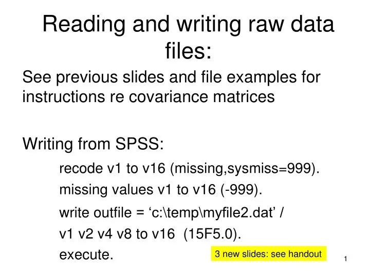
Reading and writing raw data files:. See previous slides and file examples for instructions re covariance matrices Writing from SPSS: recode v1 to v16 ( missing,sysmiss =999). missing values v1 to v16 (-999). write outfile = ‘c:tempmyfile2.dat’ / v1 v2 v4 v8 to v16 (15F5.0). execute.

E N D
Reading and writing raw data files: See previous slides and file examples for instructions re covariance matrices Writing from SPSS: recode v1 to v16 (missing,sysmiss=999). missing values v1 to v16 (-999). write outfile = ‘c:\temp\myfile2.dat’ / v1 v2 v4 v8 to v16 (15F5.0). execute. 3 new slides: see handout
SAS: libname sas2 ‘c:\temp’; location of SAS file filename out2 ‘c:\temp\rawdata1.dat’; data; set sas2.mydata; array a1 v1 -- v16; do over a1; if a1=. then a1=999; end; file out2 ls=150; put (v1 v2 v4 v5--v16)(15*10.3); run;
STATA outfile v1 v2 v4 v5-v16 using c:\temp\rawdata1.dat, nolabel wide
Reading raw data into MPlus Data: File is c:\temp\rawdata1.dat; Listwise = ON; if required; otherwise uses FIML estimation for missing data VARIABLE: Names are v1 v2 v4 v5 v6 v7 v8 v9 V10 v11 v12 v13 v14 v15 v16; Missing are ALL (999); Grouping is (1=male 2=female); <- if multiple group problem
New slide: also on file Day3(Wrapup) Two-Tailed Estimate S.E. Est./S.E. P-Value Group G1 ALC ON AGE -0.116 0.010 -11.346 0.000 EDUC 0.050 0.023 2.160 0.031 PERINC 0.191 0.041 4.700 0.000 WORK 0.266 0.071 3.741 0.000 Group 2 ALC ON AGE -0.116 0.010 -11.346 0.000 EDUC 0.050 0.023 2.160 0.031 PERINC 0.058 0.032 1.785 0.074 WORK 0.266 0.071 3.741 0.000 Estimate S.E. Est./S.E. P-Value Intercepts ALC -0.604 0.164 -3.680 0.000 MENTHLTH -2.113 0.517 -4.085 0.000 Males: Alc = 0 + .191*Perinc Females: Alc = -.604 + .058*Perinc Perinc score ranges from 1 through 6
Much trickier if more than 1 X-variable has non-parallel slope Males: Alc = 0 + .191*Perinc Females: Alc = -.604 + .058*Perinc Problem: this estimated difference would now only apply when the other X-variable(s) has a score of 0 E.g., only applicable when education = 0 Usually, we’ll want to hold other variables constant at their means. One solution: mean-centre the variables (not an issue with latent variables, where means are 0 by default in group 1; only an issue with single-indicator manifest X-variables). Or, do some additional calculations: Males: Alc = 0 + [ed coefficient [males]* mean of educ] + .191*perinc Females: Alc = -.604 + [edcoffficient[females]* mean of educ] + .058*perinc
alternative, “curve of factors” see Duncan & al, Introduction to Latent Variable Growth Curve Modeling , 1999, chapter 5 for a brief discussion zero intercept one indicator per factor **This is a new slide
factor of curves vs. curve of factors • factor of curves more parsimonious • difficult to choose from the 2 • curve of factors probably more common (for example, it is this approach that we see in Bollen and Curran, Latent Curve Models: A Structural Equation Perspective, p. 246ff.) Exercise #6 used the “curve of factors” approach, which is more common **This is a new slide
From yesterday’s exercise #6 Model: Disab1 BY move1@1; Disab2 BY move2@1 ; Disab3 BY move3@1 ; Disab1 BY sense1 (1); Disab2 BY sense2 (1); Disab3 BY sense3 (1); Disab1 BY task1 (2); Disab2 BY task2 (2); Disab3 BY task3 (2); [move1@0]; [move2@0]; [move3@0] [task1] (3); [sense1] (4); [task2] (3); [sense2] (4); [task3] (3); [sense3] (4); [Disab1@0] ; [Disab2@0]; [Disab3@0]; sense1 WITH sense2; sense2 WITH sense3; sense1 WITH sense3; Int BY Disab1@1 Disab2@1 Disab3@1; Slope BY Disab1@0 Disab2@1 Disab3@2; [Int]; [Slope]; Fix mean of 3 latent variables (one LV for each time point) to mean of move indicator) But, with LV means (technically intercepts) set to zero, values passed on to the int variable. Int variable will have mean approx = mean of move1
Means INT 4.102 0.056 73.232 0.000 SLOPE 0.279 0.024 11.393 0.000 Intercepts MOVE1 0.000 0.000 999.000 999.000 TASK1 0.259 0.059 4.366 0.000 SENSE1 1.706 0.087 19.534 0.000 MOVE2 0.000 0.000 999.000 999.000 TASK2 0.259 0.059 4.366 0.000 SENSE2 1.706 0.087 19.534 0.000 MOVE3 0.000 0.000 999.000 999.000 TASK3 0.259 0.059 4.366 0.000 SENSE3 1.706 0.087 19.534 0.000 DISAB1 0.000 0.000 999.000 999.000 DISAB2 0.000 0.000 999.000 999.000 DISAB3 0.000 0.000 999.000 999.000
An alternative parameterization Disab1 BY move1@1; Disab2 BY move2@1 ; Disab3 BY move3@1 ; Disab1 BY sense1 (1); Disab2 BY sense2 (1); Disab3 BY sense3 (1); Disab1 BY task1 (2); Disab2 BY task2 (2); Disab3 BY task3 (2); [move1] (5); [move2] (5); [move3] (5); [task1] (3); [sense1] (4); [task2] (3); [sense2] (4); [task3] (3); [sense3] (4); [Disab1@0] ; [Disab2@0]; [Disab3@0]; sense1 WITH sense2; sense2 WITH sense3; sense1 WITH sense3; Int BY Disab1@1 Disab2@1 Disab3@1; Slope BY Disab1@0 Disab2@1 Disab3@2; [Int@0]; [Slope]; task2 WITH task1; Not = 0 but equality constraints across time, just like other 2 indicators Must fix to zero
This model includes correlated errors for the sense indicator INT ON ED -0.084 0.018 -4.602 0.000 BLACK 0.575 0.230 2.504 0.012 YEARBORN 0.016 0.006 2.638 0.008 WORKING -0.600 0.147 -4.070 0.000 RETIRED -0.257 0.133 -1.927 0.054 SLOPE ON ED -0.012 0.008 -1.389 0.165 BLACK -0.183 0.106 -1.725 0.085 YEARBORN 0.009 0.003 3.032 0.002 WORKING 0.043 0.068 0.635 0.526 RETIRED 0.064 0.062 1.034 0.301
Also a gender effect:(we didn’t include gender in Ex. #6) INT ON ED -0.082 0.018 -4.476 0.000 BLACK 0.566 0.229 2.469 0.014 YEARBORN 0.015 0.006 2.458 0.014 WORKING -0.564 0.149 -3.788 0.000 RETIRED -0.208 0.137 -1.523 0.128 SEX -0.174 0.109 -1.592 0.111 SLOPE ON ED -0.010 0.008 -1.224 0.221 BLACK -0.188 0.106 -1.782 0.075 YEARBORN 0.008 0.003 2.795 0.005 WORKING 0.066 0.069 0.967 0.334 RETIRED 0.095 0.063 1.506 0.132 SEX -0.110 0.050 -2.189 0.029 Sex 1=male 0=female
A more complex model, sometimes with slopes predicting slopes • Be careful of causal order issues though INT ON YEARBORN 0.199 0.044 4.545 0.000 ED -0.230 0.044 -5.293 0.000 SEX -0.100 0.044 -2.275 0.023 SLOPE ON YEARBORN 0.260 0.062 4.181 0.000 ED -0.052 0.063 -0.823 0.411 SEX -0.113 0.062 -1.809 0.070 Int = intercept for disability Slope = slope for disability
A more complex model, sometimes with slopes predicting slopes Predicting earnings INT: EARNINT ON INT -0.159 0.043 -3.738 0.000 YEARBORN 0.004 0.052 0.075 0.940 ED 0.273 0.031 8.889 0.000 SEX 0.269 0.050 5.357 0.000 z Int = intercept for disability Slope = slope for disability
Predicting earnings slope: EARNSLOP ON INT -0.036 0.051 -0.701 0.483 SLOPE 0.015 0.083 0.175 0.861 EARNSLOP ON YEARBORN -0.130 0.061 -2.127 0.033 ED 0.107 0.035 3.112 0.002 SEX 0.089 0.058 1.530 0.126 Int = intercept for disability Slope = slope for disability
Predicting alcohol consumption slope! ALCSLOP ON INT 0.095 0.072 1.311 0.190 SLOPE -0.115 0.116 -0.990 0.322 EARNINT 0.246 0.122 2.011 0.044 EARNSLOP -0.301 0.113 -2.660 0.008 YEARBORN -0.125 0.086 -1.455 0.146 ED -0.031 0.055 -0.552 0.581 SEX -0.010 0.083 -0.121 0.904 Int = intercept for disability Slope = slope for disability
piecewise latent curve model not shown: 0 path (not needed!) from slope2 to v1-t1, v1-t2 parm33RM Slope1: change from time 1 through time 3 Slope 2: Change from time 3 through time 5 New slide not previously discussed