Review – Using Standard Deviation

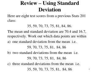
Review – Using Standard Deviation Here are eight test scores from a previous Stats 201 class: 35, 59, 70, 73, 75, 81, 84, 86. The mean and standard deviation are 70.4 and 16.7, respectively. Work out which data points are within • one standard deviation from the mean i.e. 59,70, 73, 75, 81, 84, 86 • two standard deviations from the mean i.e. 59, 70, 73, 75, 81, 84, 86 c) three standard deviations from the mean i.e. 35, 59, 70, 73, 75, 81, 84, 86

Idea! • The example suggests that there may be a general rule which allows us to estimate the fraction of data points which are within a given number of standard deviations of the mean.

Distribution curves If the number of data points n is small, one uses a small number of class intervals and obtains a typical histogram

Histogram (small n)

Distribution curves If the number of data points n is lager, one can use more subintervals in producing a histogram for the data set

Histogram (Medium n)

Distribution curves If the number of data points n is very large, one can use a corresponding large number of class intervals and obtain a histogram which cn be seen to approach a curve in the limit as n increases. In this case, it is convenient to choose the scale on the vertical axis so that the area of each vertical bar corresponds to the fraction of data poins in the corresponding subinterval. NOTE: The total area under the graph of the histogram will therefore be 1.

Histogram (large n)

In the limit as the size of the population increases, one obtains a smooth curve. This curve was called a probability density function in Math 112 One obtains different curves corresponding to different population means and variances.

Normal Distributions Shape of this curve is determined by µ and σ • µ it’s centered, σ is how far it’s spread out.

Interpreting the Standard Deviation Chebyshev’s Theorem The proportion (or fraction) of any data set lying within K standard deviations of the mean is always at least 1-1/K2, where K is any positive number greater than 1. For K=2 we obtain, at least 3/4 (75 %) of all scores will fall within 2 standard deviations of the mean, i.e. 75% of the data will fall between

Interpreting the Standard Deviation Chebyshev’s Theorem The proportion (or fraction) of any data set lying within K standard deviations of the mean is always at least 1-1/K2, where K is any positive number greater than 1. For K=3 we obtain, at least 8/9 (89 %) of all scores will fall within 3 standard deviations of the mean, i.e. 89% of the data will fall between

Exercise 1 • Data collected daily at an intersection giving the number of cars passing through. • Mean = 375 with standard deviation 25 • Estimate the fraction of days that more than 425 cars used the intersection.

Exercise 1 • Data collected daily at an intersection giving the number of cars passing through. • Mean = 375 with standard deviation 25 • Estimate the fraction of days that more than 425 cars used the intersection. • ANS: At least 75% lie in the interval (325, 425). Therefore, at most 25% lie outside this interval.

Exercise 1 • NOTE: Assuming the data is symmetric and therefore evenly distributed about the mean, we can conclude that the 25% which lie outside the interval (325,425) are evenly distributed into 12.5% lying above 425 and 12.5% lying below 3.25. 5, 425). Therefore, on roughly 12.5% of the days there will be more than 425 cars using the intersection.

If the data is known to have a histogram which is symmetric about the mean and “bell shaped”, one can improve upon Chebyshev’s Rule

This Data is Symmetric, Bell Shaped (or Normal Data) Relative Frequency 0.5 0.4 0.3 0.2 0.1 1 2 3 4 5 0

This Data is Symmetric, Bell Shaped (or Normal Data) Relative Frequency 0.5 0.4 0.3 0.2 0.1 1 2 3 4 5 7 0 6

The Empirical Rule The Empirical Rule states that for bell shaped (normal) data: 68% of all data points are within 1 standard deviations of the mean 95% of all data points are within 2 standard deviations of the mean 99.7% of all data points are within 3 standard deviations of the mean

The Empirical Rule The Empirical Rule states that for bell shaped (normal) data, approximately: 68% of all data points are within 1 standard deviations of the mean 95% of all data points are within 2 standard deviations of the mean 99.7% of all data points are within 3 standard deviations of the mean

Exercise 2 • Data collected daily at an intersection giving the number of cars passing through. • Mean = 375 with standard deviation 25 • Estimate the fraction of days that more than 425 cars used the intersection assuming the data is bell-shaped.

Exercise 2 • Data collected daily at an intersection giving the number of cars passing through. • Mean = 375 with standard deviation 25 • Estimate the fraction of days that more than 425 cars used the intersection assuming the data is bell-shaped. • ANS: 2.5% (Check this!)

Z-Score To calculate the number of standard deviations a particular point is away from the standard deviation we use the following formula.

Z-Score To calculate the number of standard deviations a particular point is away from the standard deviation we use the following formula. The number we calculate is called the z-score of the measurement x.

Example – Z-score Here are eight test scores from a previous Stats 201 class: 35, 59, 70, 73, 75, 81, 84, 86. The mean and standard deviation are 70.4 and 16.7, respectively. a) Find the z-score of the data point 35. b) Find the z-score of the data point 73.

Example – Z-score Here are eight test scores from a previous Stats 201 class: 35, 59, 70, 73, 75, 81, 84, 86. The mean and standard deviation are 70.4 and 16.7, respectively. • Find the z-score of the data point 35. z = -2.11 b) Find the z-score of the data point 73. z = 0.16

Interpreting Z-scores The further away the z-score is from zero the more exceptional the original score. Values of z less than -2 or greater than +2 can be considered exceptional or unusual (“a suspected outlier”). Values of z less than -3 or greater than +3 are often exceptional or unusual (“a highly suspected outlier”).

Example: Aptitude tests Before being accepted into a manufacturing job, one must complete two aptitude tests. Your score on the tests will decide whether you will be in management or whether you will work on the factory floor. One test is a manual dexterity test, the other is a statistics test. The manual dexterity test (out of 10) has a mean of 6 and a standard deviation of 1. The statistics test (out of 50) has a mean of 25 with a standard deviation of 3. Your score is 7/10 on the manual dexterity test, and a 34/50 on the statistics test. In which test were you exceptional?

The problem with comparing the two test scores stems from the fact that the tests are on two different scales. If we are going to do meaningful comparisons, then we must somehow, standardize the scores. Example: Aptitude tests

Answer Calculate the z-score for the two tests. • Z-score of Man. Dex. = (7-6)/1 = 1 • Z-score of Stats. = (34-25)/3 = 3 Your score on the stats test was exceptionally high (3 standard deviations above the mean.

Review – Using Standard Deviation