Advanced Signal Deconvolution Techniques for fMRI Analysis
Explore deconvolution methods to model brain activity in fMRI data, from fixed-shape regression to variable shapes. Learn about pros and cons, expressing HRF via regression, using tent functions, and more.

Advanced Signal Deconvolution Techniques for fMRI Analysis
E N D
Presentation Transcript
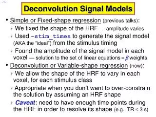
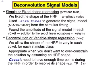
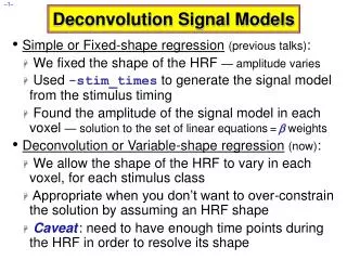
Deconvolution Signal Models • Simple or Fixed-shape regression(previous talks): • We fixed the shape of the HRF — amplitude varies • Used -stim_times to generate the signal model from the stimulus timing • Found the amplitude of the signal model in each voxel — solution to the set of linear equations= weights • Deconvolution or Variable-shape regression(now): • We allow the shape of the HRF to vary in each voxel, for each stimulus class • Appropriate when you don’t want to over-constrain the solution by assuming an HRF shape • Caveat: need to have enough time points during the HRF in order to resolve its shape
Deconvolution: Pros & Cons (+ & –) • Letting HRF shape varies allows for subject and regional variability in hemodynamics • Can test HRF estimate for different shapes (e.g., are later time points more “active” than earlier?) • Need to estimate more parameters for each stimulus class than a fixed-shape model (e.g., 4-15 vs. 1 parameter=amplitude of HRF) • Which means you need more data to get the same statistical power (assuming that the fixed-shape model you would otherwise use was in fact “correct”) • Freedom to get any shape in HRF results can give weird shapes that are difficult to interpret
Expressing HRF via Regression Unknowns • The tool for expressing an unknown function as a finite set of numbers that can be fit via linear regression is an expansion in basis functions • The basis functions q(t) & expansion order p are known • Larger p more complex shapes & more parameters • The unknowns to be found (in each voxel) comprises the set of weightsqfor each q(t) • weights appear only by multiplying known values, and HRF only appears in signal model by linear convolution (addition) with known stimulus timing • Resulting signal model still solvable by linear regression
3dDeconvolve with “Tent Functions” • Need to describe HRF shape and magnitude with a finite number of parameters • And allow for calculation of h(t) at any arbitrary point in time after the stimulus times: • Simplest set of such functions are tent functions • Also known as “piecewise linear splines” h time t=0 t=TR t=2TR t=3TR t=4TR t=5TR
A Tent Functions = Linear Interpolation • Expansion of HRF in a set of spaced-apart tent functions is the same as linear interpolation between “knots” • Tent function parameters are also easily interpreted as function values (e.g., 2 = response at time t = 2L after stim) • User must decide on relationship of tent function grid spacing L and time grid spacing TR (usually would choose L TR) • In 3dDeconvolve: specify duration of HRF and number of parameters (details shown a few slides ahead) h 2 3 N.B.: 5 intervals = 6 weights 1 4 0 5 time “knot” times 0 L 2L 3L 4L 5L
Tent Functions: Average Signal Change • For input to group analysis, usually want to compute average signal change • Over entire duration of HRF (usual) • Over a sub-interval of the HRF duration (sometimes) • In previous slide, with 6 weights, average signal change is 1/2 0 +1 +2 +3 +4 +1/2 5 • First and last weights are scaled by half since they only affect half as much of the duration of the response • In practice, may want to use 00 since immediate post-stimulus response is not neuro-hemodynamically relevant • All weights (for each stimulus class) are output into the “bucket” dataset produced by 3dDeconvolve • Can then be combined into a single number using 3dcalc
0 +4 0 +4 0 +4 1 +5 1 +5 1 +5 3 3 3 2 2 2 Equations at each data time point: Cannot tell 0 from 4, or 1 from 5 0 1 2 3 HRF from stim #1 0 0 0 1 1 1 2 2 2 3 3 3 4 4 4 5 5 5 A stim #1 Deconvolution and Collinearity • Regular stimulus timing can lead to collinearity! time Tail of HRF from #1 overlaps head of HRF from #2, etc
Deconvolution Example - The Data • cd AFNI_data2 • data is in ED/ subdirectory (10 runs of 136 images each; TR=2 s) • script = s1.afni_proc_command(in AFNI_data2/ directory) • stimuli timing and GLT contrast files in misc_files/ • this script runs program afni_proc.py to generate a shell script with all AFNI commands for single-subject analysis • Run by typing tcsh s1.afni_proc_command; then copy/paste tcsh -x proc.ED.8.glt |& tee output.proc.ED.8.glt • Event-related study from Mike Beauchamp • 10 runs with four classes of stimuli (short videos) • Tools moving (e.g., a hammer pounding) - ToolMovie • People moving (e.g., jumping jacks) - HumanMovie • Points outlining tools moving (no objects, just points) - ToolPoint • Points outlining people moving - HumanPoint • Goal: find brain area that distinguishes natural motions (HumanMovie and HumanPoint) from simpler rigid motions (ToolMovie and ToolPoint) Text output from programs goes to screen andfile
Master Script for Data Analysis • Master script program • 10 input datasets • Set output filenames • Copy anat to output dir • Discard first 2 TRs • Where to align all EPIs • Stimulus timing files (4) • Stimulus labels • HRF model • Specifies that next lines are options to be passed to 3dDeconvolve directly (in this case, the GLTs we want computed) afni_proc.py \ -dsets ED/ED_r??+orig.HEAD \ -subj_id ED.8.glt \ -copy_anat ED/EDspgr \ -tcat_remove_first_trs 2 \ -volreg_align_to first \ -regress_stim_times misc_files/stim_times.*.1D \ -regress_stim_labels ToolMovie HumanMovie \ ToolPoint HumanPoint \ -regress_basis 'TENT(0,14,8)' \ -regress_opts_3dD \ -gltsym ../misc_files/glt1.txt -glt_label 1 FullF \ -gltsym ../misc_files/glt2.txt -glt_label 2 HvsT \ -gltsym ../misc_files/glt3.txt -glt_label 3 MvsP \ -gltsym ../misc_files/glt4.txt -glt_label 4 HMvsHP \ -gltsym ../misc_files/glt5.txt -glt_label 5 TMvsTP \ -gltsym ../misc_files/glt6.txt -glt_label 6 HPvsTP \ -gltsym ../misc_files/glt7.txt -glt_label 7 HMvsTM } This script generates file proc.ED.8.glt(180 lines), which contains all the AFNI commands to produce analysis results into directory ED.8.glt.results/ (148 files)
Shell Script for Deconvolution - Outline • Copy datasets into output directory for processing • Examine each imaging run for outliers: 3dToutcount • Time shift each run’s slices to a common origin: 3dTshift • Registration of each imaging run: 3dvolreg • Smooth each volume in space (136 sub-bricks per run): 3dmerge • Create a brain mask: 3dAutomask and 3dcalc • Rescale each voxel time series in each imaging run so that its average through time is 100: 3dTstat and 3dcalc • If baseline is 100, then a q of 5 (say) indicates a 5% signal change in that voxel at tent function knot #q after stimulus • Biophysics: believe % signal change is relevant physiological parameter • Catenate all imaging runs together into one big dataset (1360 time points): 3dTcat • This dataset is useful for plotting -fitts output from 3dDeconvolve and visually examining time series fitting • Compute HRFs and statistics: 3dDeconvolve
Script - 3dToutcount # set list of runs set runs = (`count -digits 2 1 10`) # run 3dToutcount for each run foreach run ( $runs ) 3dToutcount -automask pb00.$subj.r$run.tcat+orig > outcount_r$run.1D end Via 1dplot outcount_r??.1D 3dToutcount searches for “outliers” in data time series; You may want to examine noticeable runs & time points
Script - 3dTshift # run 3dTshift for each run foreach run ( $runs ) 3dTshift -tzero 0 -quintic -prefix pb01.$subj.r$run.tshift \ pb00.$subj.r$run.tcat+orig end • Produces new datasets where each time series has been shifted to have the same time origin • -tzero 0 means that all data time series are interpolated to match the time offset of the first slice • Which is what the slice timing files usually refer to • Quintic (5th order) polynomial interpolation is used • 3dDeconvolve will be run on time-shifted datasets • This is mostly important for Event-Related FMRI studies, where the response to the stimulus is briefer than for Block designs • (Because the stimulus is briefer) • Being a little off in the stimulus timing in a Block design is not likely to matter much
Script - 3dvolreg # align each dset to the base volume foreach run ( $runs ) 3dvolreg -verbose -zpad 1 -base pb01.$subj.r01.tshift+orig'[0]' \ -1Dfile dfile.r$run.1D -prefix pb02.$subj.r$run.volreg \ pb01.$subj.r$run.tshift+orig end • Produces new datasets where each volume (one time point) has been aligned (registered) to the #0 time point in the #1 dataset • Movement parameters are saved into files dfile.r$run.1D • Will be used as extra regressors in 3dDeconvolveto reduce motion artifacts • 1dplot -volreg dfile.rall.1D • Shows movement parameters for all runs (1360 time points) in degrees and millimeters • Important to look at this graph! • Excessive movement can make an imaging run useless — 3dvolreg won’t be able to compensate • Pay attention to scale of movements: more than about 2 voxel sizes in a short time interval is usually bad
Script - 3dmerge # blur each volume foreach run ( $runs ) 3dmerge -1blur_fwhm 4 -doall -prefix pb03.$subj.r$run.blur \ pb02.$subj.r$run.volreg+orig end • Why Blur? Reduce noise by averaging neighboring voxels time series • White curve = Data: unsmoothed • Yellow curve = Model fit (R2=0.50) • Green curve = Stimulus timing This is an extremely good fit for ER FMRI data!
Why Blur? - 2 • fMRI activations are (usually) blob-ish (several voxels across) • Averaging neighbors will also reduce the fiendish multiple comparisons problem • Number of independent “resels” will be smaller than number of voxels (e.g., 2000 vs. 20000) • Why not just acquire at lower resolution? • To avoid averaging across brain/non-brain interfaces • To project onto surface models • Amount to blur is specified as FWHM (Full Width at Half Maximum) of spatial averaging filter (4 mm in script)
Script - 3dAutomask # create 'full_mask' dataset (union mask) foreach run ( $runs ) 3dAutomask -dilate 1 -prefix rm.mask_r$run pb03.$subj.r$run.blur+orig end # get mean and compare it to 0 for taking 'union' 3dMean -datum short -prefix rm.mean rm.mask*.HEAD 3dcalc -a rm.mean+orig -expr 'ispositive(a-0)' -prefix full_mask.$subj • 3dAutomask creates a mask of contiguous high-intensity voxels (with some hole-filling) from each imaging run separately • 3dMean and 3dcalc are used to create a mask that is the union of all the individual run masks • 3dDeconvolve analysis will be limited to voxels in this mask • Will run faster, since less data to process
Script - Scaling # scale each voxel time series to have a mean of 100 # (subject to maximum value of 200) foreach run ( $runs ) 3dTstat -prefix rm.mean_r$run pb03.$subj.r$run.blur+orig 3dcalc -a pb03.$subj.r$run.blur+orig -b rm.mean_r$run+orig \ -c full_mask.$subj+orig \ -expr 'c * min(200, a/b*100)' -prefix pb04.$subj.r$run.scale end • 3dTstat calculates the mean (through time) of each voxel’s time series data • For voxels in the mask, each data point is scaled (multiplied) using 3dcalc so that it’s time series will have mean=100 • If an HRF regressor has max amplitude=1, then its coefficient will represent the percent signal change (from the mean) due to that part of the signal model • Scaled images are very boring • No spatial contrast by design! • Graphs have common baseline now
Script - 3dDeconvolve } 3dDeconvolve -input pb04.$subj.r??.scale+orig.HEAD -polort 2 \ -mask full_mask.$subj+orig -basis_normall 1 -num_stimts 10 \ -stim_times 1 stimuli/stim_times.01.1D 'TENT(0,14,8)' \ -stim_label 1 ToolMovie \ -stim_times 2 stimuli/stim_times.02.1D 'TENT(0,14,8)' \ -stim_label 2 HumanMovie \ -stim_times 3 stimuli/stim_times.03.1D 'TENT(0,14,8)' \ -stim_label 3 ToolPoint \ -stim_times 4 stimuli/stim_times.04.1D 'TENT(0,14,8)' \ -stim_label 4 HumanPoint \ -stim_file 5 dfile.rall.1D'[0]' -stim_base 5 -stim_label 5 roll \ -stim_file 6 dfile.rall.1D'[1]' -stim_base 6 -stim_label 6 pitch \ -stim_file 7 dfile.rall.1D'[2]' -stim_base 7 -stim_label 7 yaw \ -stim_file 8 dfile.rall.1D'[3]' -stim_base 8 -stim_label 8 dS \ -stim_file 9 dfile.rall.1D'[4]' -stim_base 9 -stim_label 9 dL \ -stim_file 10 dfile.rall.1D'[5]' -stim_base 10 -stim_label 10 dP \ -iresp 1 iresp_ToolMovie.$subj -iresp 2 iresp_HumanMovie.$subj \ -iresp 3 iresp_ToolPoint.$subj -iresp 4 iresp_HumanPoint.$subj \ -gltsym ../misc_files/glt1.txt -glt_label 1 FullF \ -gltsym ../misc_files/glt2.txt -glt_label 2 HvsT \ -gltsym ../misc_files/glt3.txt -glt_label 3 MvsP \ -gltsym ../misc_files/glt4.txt -glt_label 4 HMvsHP \ -gltsym ../misc_files/glt5.txt -glt_label 5 TMvsTP \ -gltsym ../misc_files/glt6.txt -glt_label 6 HPvsTP \ -gltsym ../misc_files/glt7.txt -glt_label 7 HMvsTM \ -fout -tout -full_first -x1D Xmat.x1D -fitts fitts.$subj -bucket stats.$subj 4 stim types } motion params } HRF outputs } GLTs
Results: Humans vs. Tools • Color overlay: HvsT GLT contrast • Blue(upper) graphs: Human HRFs • Red(lower) graphs: Tool HRFs
Script - X Matrix Via 1grayplot -sep Xmat.x1D
Script - Random Comments • -polort 2 • Sets baseline (detrending) to use quadratic polynomials—in each run • -mask full_mask.$subj+orig • Process only the voxels that are nonzero in this mask dataset • -basis_normall 1 • Make sure that the basis functions used in the HRF expansion all have maximum magnitude=1 • -stim_times 1 stimuli/stim_times.01.1D 'TENT(0,14,8)' -stim_label 1 ToolMovie • The HRF model for the ToolMovie stimuli starts at 0 s after each stimulus, lasts for 14 s, and has 8 basis tent functions • Which have knots spaced 14/(8-1)=2 s apart) • -iresp 1 iresp_ToolMovie.$subj • The HRF model for the ToolMovie stimuli is output into dataset iresp_ToolMovie.ED.8.glt+orig
Script - GLTs • -gltsym ../misc_files/glt2.txt -glt_label 2 HvsT • File ../misc_files/glt2.txt contains 1 line of text: • -ToolMovie +HumanMovie -ToolPoint +HumanPoint • This is the “Humans vs. Tools” HvsT contrast shown on Results slide • This GLT means to take all 8 coefficients for each stimulus class and combine them with additions and subtractions as ordered: • This test is looking at the integrated (summed) response to the “Human” stimuli and subtracting it from the integrated response to the “Tool” stimuli • Combining subsets of the weights is also possible with -gltsym: • +HumanMovie[2..6] -HumanPoint[2..6] • This GLT would add up just the #2,3,4,5, & 6 weights for one type of stimulus and subtract the sum of the #2,3,4,5, & 6 weights for another type of stimulus • And also produce F- and t-statistics for this linear combination
+ToolMovie +HumanMovie +ToolPoint +HumanPoint 4 rows Script - Multi-Row GLTs • GLTs presented up to now have had one row • Testing if some linear combination of weights is nonzero; test statistic is t or F (F=t2 when testing a single number) • Testing if the X matrix columns, when added together to form one column as specified by the GLT (+ and –), explain a significant fraction of the data time series (equivalent to above) • Can also do a single test to see if several different combinations of weights are all zero -gltsym ../misc_files/glt1.txt -glt_label 1 FullF • Tests if any of the stimulus classes have nonzero integrated HRF (each name means “add up those weights”) : DOF= (4,1292) • Different than the default “Full F-stat” produced by 3dDeconvolve, which tests if any of the individual weights are nonzero: DOF= (32,1292)
Two Possible Formats for -stim_times 4.7 9.6 11.8 19.4 • A single column of numbers (GLOBAL times) • One stimulus time per row • Times are relative to first image in dataset being at t=0 • May not be simplest to use if multiple runs are catenated • One row for each run within a catenated dataset (LOCAL times) • Each time in jth row is relative to start of run #j being t=0 • If some run has NO stimuli in the given class, just put a single “*” in that row as a filler • Different numbers of stimuli per run are OK • At least one row must have more than 1 time (so that the LOCAL type of timing file can be told from the GLOBAL) • Two methods are available because of users’ diverse needs • N.B.: if you chop first few images off the start of each run, the inputs to -stim_times must be adjusted accordingly! 4.7 9.6 11.8 19.4 * 8.3 10.6